Page Contents

Overview

In our study of Quality of Service (QoS) in packet networks we will be concerned with measures such as delay, delay variation, packet loss, and bandwidth/throughput. As a network and particularly an individual link has a finite amount of bandwidth we will be concerned with how this bandwidth gets allocated among users and their corresponding flows. An important question that goes far beyond just the technical aspects that we will cover here is: who gets what type of QoS and in particular how much of limited bandwidth resources? In addition, if there is excess bandwidth capacity how should it be fairly allocated?

Some of the concepts we will be studying are the most important where bandwidth is the least plentyful such as at the network edge or on access links, e.g., between home or small business networks and their internet service provider. In fact almost all the practical mechanisms that we shall discuss in the following text are available within the core of Linux networking and available in open source compatible wireless routers via the OpenWRT project.

One way to characterize the mechanisms use to provide QoS is by looking at the different time scales that they operate:

Years or Months

: Network Provisioning, Lighting new wavelengths, etc...

Minutes or Less

: Flow admission Control/Resource, Reservation/Path Computation

Multiple down to Single Packet Duration

: Traffic Policing, Traffic Shaping, Queueing Disciplines

Another way to look at mechanisms that provide for QoS is based on the network domain or scope at which they operate:

Network wide : network provisioning, admision control, resource reservation

Subnetwork : admission control, resource reservation, policing, shaping

Per Link : Packet scheduling, active queue management, policing, shaping

In the following we will primarily be concerned with the shorter duration subnet and per link mechanisms for providing QoS.

Characterizing Traffic

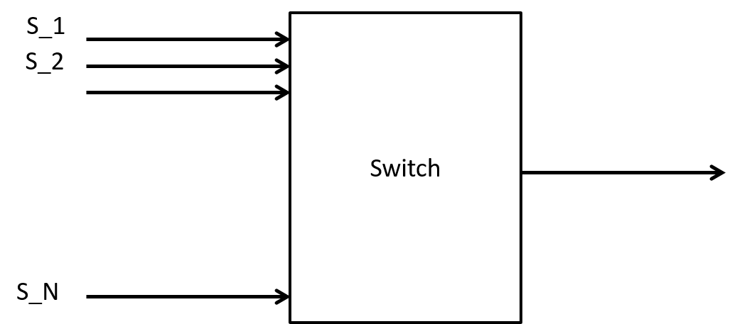
Let’s revisit our earlier packet switch example, shown in Figure 1.

Figure 1. A many input switch for study.

Example:

Consider $N=100$ sources, $S_i$ sending constant bit rate traffic (say video) over a packet network. Suppose that the packet size, L, is constant and $L= 1250 \text{ bytes} = 10,000 \text{ bits}$. If the sources have an average bit rate of $r = 5\text{Mbps}$ per second they will send a packet every $1.0\times10^4 \text{bits}/5.0\times 10^6\text{bps} = 2\text{mS}$.

Suppose we have a 101 port Ethernet (1Gbps per port) switch connected with a server that is supposed to receive all these video streams. How big or small could the output queue for this one port get? In terms of the number of packets? Or in terms of the number of bytes?

First we compute how long it takes to transmit one of these packets on a 1Gbps port. Answer: $1.0\times 10^4 \text{bits}/1.0\times 10^9 \text{bps} = 1.0 \times 10^{-5}= 10 \mu s$. Next we compute the packet rate: $\text{Packet rate} = r/L = 500 \text{packets/sec}$.

Since we have to send one of these packets every 2ms, how many different streams can we send? $\text{Answer} = 2ms/10\mu s = 200$. Or we can think of each 1Gbps link having the equivalent of 200 packet arrival slots per 2ms.

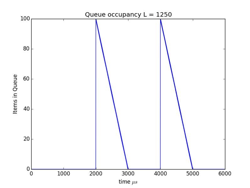
If the senders are all synchronized what is the maximum queue in bytes that can build up? Worst case Queue size in bytes = (N)(L).

How long does it take for the queue to drain? What is the maximal delay? $$Delay = NL/C$$

Queue builds up and drains away in a periodic manner! As shown in Figure 2. So far we have dealt with two important traffic parameters:

Average rate : Is the number of bits sent by a source divided by the time. Generally the time is taken to be quite long compared to the line rate of the source. In our current example the average rate of the sources is 5Mbps.

Peak rate : Is the maximum rate at which a packet or packets are sent. In our example the peak rate was just the line rate of the link. In general this can be much lower than the line rate. In such a case the peak rate is actually an average taken over a much shorter time period than the average rate.

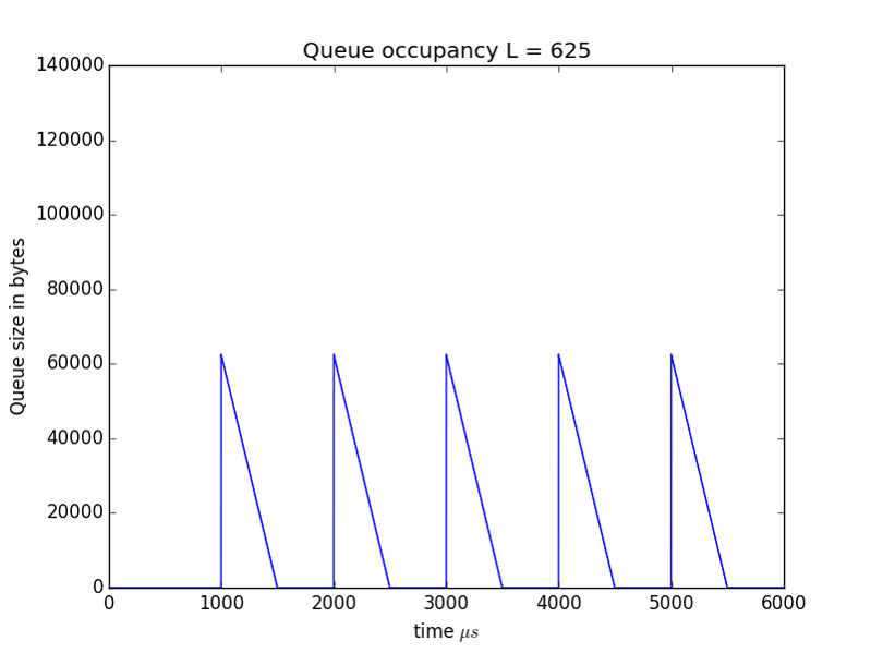
Figure 2. Queue size over time in packets L=1250.

In Figure 3 we show the effect of cutting the packet size in half. To keep the average 5Mpbs rate the sources need to send twice as often so we see more frequent peaks in the queue size. At first it would appear we've gained little benefit from the reduction in packet size, but recall from above $Delay = NL/C$ so cutting the packet size in half cut the maximum delay seen by one half.

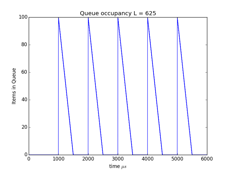
Figure 3. Queue size over time in packets L=625.

To make this clearer in Figures 4 and 5 we show the queue sizes in bytes rather than packets for the cases of $L=1250$ and $L=625$ respectively.

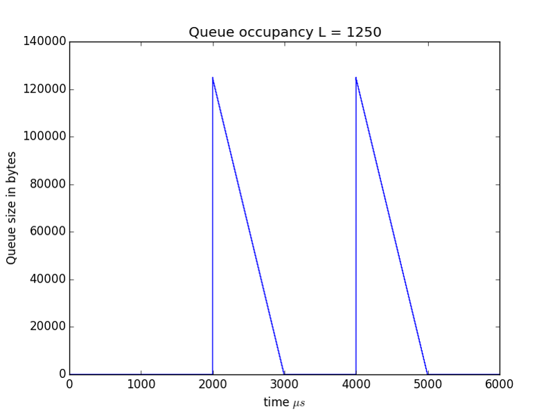
Figure 4. Queue size over time in *bytes* L=1250.

Figure 5. Queue size over time in *packets* L=625.

This would seem to indicate that another traffic parameter may be useful:

Maximum Burst Size : The maximum burst size (MBS) for a traffic flow is the largest number of bytes that a source sends contiguously at the peak rate. We see in our simple constant bit rate, constant packet size example that this was simply the packet length in bytes.

What is the smallest burst size possible (not worrying about packet overhead)? → 1 byte or even 1 bit.

If we use that how would our worst case delay and buffer size compare with circuit switching? → It would become the same as in circuit switching.

In general why do we want L large? → reduce wasted bandwidth due to packet overhead.

Networks and QoS Survey

In the older telephone network quality (QoS) of service focused on voice quality and the probability of call blocking. Before we dig into the details of QoS analysis and implementation we quickly survey some of the QoS features introduced in various packet switching technologies both historical and current. Do not worry about the exact terminology used by a particular technology we will later go over the general concepts and where useful look at precise definitions from standards development organizations.

Frame Relay

As a predicessor to both ATM and MPLS frame relay introduced a number of key packet traffic characterization measures. As an example here is an excerpt from the Wikipedia entry on frame relay's committed information rate parameter:

“Frame relay connections are often given a committed information rate (CIR) and an allowance of burstable bandwidth known as the extended information rate (EIR). The provider guarantees that the connection will always support the CIR rate, and sometimes the PIR rate should there be adequate bandwidth. Frames that are sent in excess of the CIR are marked as discard eligible (DE) which means they can be dropped should congestion occur within the frame relay network. Frames sent in excess of the EIR are dropped immediately. All traffic exceeding the CIR is marked discard eligible.”

Key Concepts from frame relays: committed (guaranteed) information rate, excess or peak rate, and burstable bandwidth.

ATM

Asynchronous Transfer Mode utilized many of the frame relay traffic parameters, suitably adjusted for ATM's fixed packet length. Like frame relay it had the notion of traffic contracts. ATM had the following types of service:

CBR - Constant bit rate: a Peak Cell Rate (PCR) is specified, which is constant.
VBR - Variable bit rate: an average or Sustainable Cell Rate (SCR) is specified, which can peak at a certain level, a PCR, for a maximum interval before being problematic.
ABR - Available bit rate: a minimum guaranteed rate is specified.
UBR - Unspecified bit rate: traffic is allocated to all remaining transmission capacity.

Other ATM traffic concepts: Policing (generic cell rate algorithm GCRA), Cell Loss Priority (CLP), Traffic Shaping.

Ethernet

IEEE Standards say very little about QoS but do give up three bits known as the priority code point (PCP) to use as shown in Figure 6 from IEEE 802.1Q-2014.

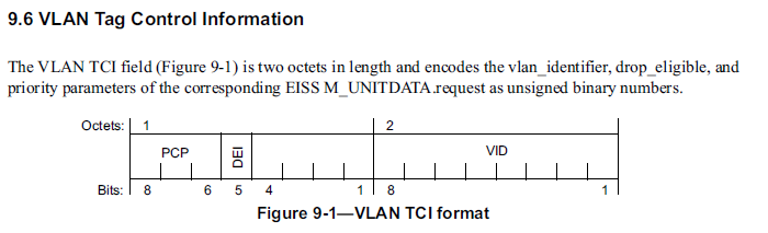
Where PCP = Priority Code Point, DEI = Drop Eligibility Indicator, VID = VLAN Identifier. Both PCP and DEI can be useful as part of a QoS regime.

Metro Ethernet Forum and Ethernet QoS

Frame relay and ATM are antiquated technologies but similar (almost exactly the same) techniques can be applied to Ethernet services. Precise and up to date definitions of performance measures and traffic profiles were created by the Metro Ethernet Forum and can be found in MEF Technical Specification MEF 10.3, "Ethernet Services Attributes Phase 3". See section 8.8 of MEF 10.3 for performance service attributes. See section 12 for bandwidth profiles.

IP and MPLS

IP started its existence as a "Best effort" technology with no particular QoS measures or traffic parameters. The IPv4 header contained "Type of Service" bits but these were not widely usedand have since been repurposed (some to QoS). The Integrated Services Internet of the mid 1990's contained a number of very good concepts but was never deployed. The Differentiated Services internet model of the late 1990's took a more practical approach and is frequently used in intranets (though not the Internet as a whole).

MPLS makes use of Integrated Services models via RSVP-TE and Differentiated Services models/concepts. We’ll go over Integrated and Differentiated services architectures after we have learned more of the concepts and mechanisms for providing QoS.

QoS Guarantees: Delays and Queues

In our first look at QoS we will look at two ways of furnishing QoS guarantees with respect to queueing induced delays. The first method is statistical and is based on the queueing theory we previously studied. The second approach obtains worst case bounds in a more general way than our 100 CBR source example in the introduction.

Statistical

From the statistical poinf of view we have some aggregate limit theorems. These are similar to the central limit theorem except that they apply to stochastic processes.

From reference [Arfeen2013]:

"Cox’s superposition theorem (1954) can be used to describe traffic at high multiplexing levels. He considered the superposition of $n$ independent renewal sequences and proved that as $n \rightarrow \infty$, the count process in the superposed sequence tends to Poisson and corresponding inter-arrival distribution tends to exponential."

"For finite n, Cinlar and Dudley (1972) showed that the rate of convergence in distribution to Poisson is $1/n$."

Where/when would such results be useful? In places where lots of packet streams get aggregated, e.g., the network core. In such cases our previous M/M/1, M/M/1/k queueing results based on Poisson traffic would be useful. These would then be used to give the probability that a delay would exceed a given bound and other useful statistical measures.

Hard Bounds on Delays and Queues

Idea: "In an ideal world well behaved traffic would get well behaved delays". But how do we make these notions precise? In the following we outline the approach from [Cruz1991]. For consistency with [Cruz1991] we will use the term traffic stream which is essentially the same as the general idea of traffic flow we have used when discussing MPLS and SDNs.

Definition (Traffic Stream) A traffic stream consists of a collection of possibly variable length packets with maximum length L.

Definition (Rate) $R(t)$ is the instantaneous rate of a traffic stream if the amount of data sent on the interval $[x, y]$ is given by $$Data[x,y] = \int\limits_x^y {R(t)dt} $$

$R(t)$ is called the rate function of the stream.

Notes: For modeling purposes sometimes $\delta(\cdot)$ functions can be used to approximate very fast links. In addition, one can make a "fluid approximation" if we allow packets to be infinitely divisible, i.e., with $L=0$ but we will not worry about those cases here.

Restrictions If $L>0$ and $C$ is the link rate in bits per second then $R(t) \in {0, C}$.

Definition (Constrained Flow) Given $\sigma \geq 0$ and $\rho \geq 0$ then then we say that $R(t) \sim (\sigma, \rho)$ is (s, r), i.e., $R(t)$ is $(\sigma, \rho)$ constrained, if and only if for all $x, y$ satisfying $y \geq x$:

$$\int\limits_x^y {R(t)dt} \leq \sigma + \rho (y - x)$$

Intuitively we can think of $\rho$ as an upper bound on the long term average rate of the source and $\sigma$ as an upper bound on the burst size. In addition we get an upper bound of $\sigma + \rho(y-x)$ for the traffic sent during the interval $[x, y]$.

Definition (work conserving system) A queueing system is called work conserving if it sends a packet whenever capacity is available on the link and there is a packet in the queueing system.

Non-work conserving systems may hold packets that could be sent to achieve some goal or to simplify the implementation of a queueing discipline.

Definition (backlogged work) The (worst case) backlogged work (or backlogged traffic) at time $t$ with input $R(t)$ and rate $\rho$, denoted $W_\rho (t)$, is given by $${W_\rho }(R)(t) = \max_{s \leq t} \left[ {\int\limits_s^t {R(x)dx - } \rho (t - s)} \right] \tag{Backlog}$$

for $- \infty < t < \infty$.

Note ${W_\rho }(R)(t) \leq \sigma$ for all t if and only if $R\sim(\sigma ,\rho )$. We can interpret this as the backlog (unsent packets) at a server with rate $\rho$.

Example Let there be two inputs to a work conserving system with rates $R_1(t)$ and $R_2(t)$. Let the output of the system have a rate $C_0$ then

(1) The input rate function to the system is just $R_1 + R_2$ (2) The Backlog in the system at time $t$ is $W_{C_0}(R_1 + R_2)(t)$.

As is frequently done in practice more general constraints on streams can be defined. In general if $b(\cdot)$ is a function on $\mathbb{R}^+$ then we say $R \sim b$ if $$\int_x^y {R(t)dt} \leq b(y-x)$$

Analysis of a Multiplexer

To analyze and bound the delays in a network we need an analytic model for a multiplexer. We use the following definition from [Cruz1991]. Let $n$ denote the number of inputs to a multiplexer and $C_i$ the rate of input link $i$. Let $C_{out}$ denote the rate of the output link of the multiplexer. We will require that $C_i \geq C_{out}$ for all $i$. Our multiplexer will use a first come first served (FCFS) queueing discipline and will start to send a packet as soon as the first bit is received which is why we need the condition on the input line rates. This behavior is shown in the figure below for a two input multiplexer from [Cruz1991]. In this figure all inputs and output links have rate $C$ and each input sends two packets labeled 1 and 2. The rate functions for the inputs and output are shown and well as the "backlog" $B(t)$.

Two input multiplexer model from [Cruz1991]

You may be thinking that the requirement for $C_i \geq C_{out}$ is quite odd since we encounter many cases in practice where this is not true. Such a constraint allowed for the modeling of cut-through switching which was popular in the early days of packet switching where link speeds were extremely slow compared to today. In cut-through switching one could start sending a packet out an egress link before it was completely received on an ingress link. This was useful when maximizing link utilization and minimizing buffer space when going from fast LAN links to relatively slow WAN links. To model more conventional packet switching, in olden times referred to as store and forward, [Cruz1991] introduces an additional modeling component that they call a receive buffer and combines that with this multiplexer model. We will not go into that level of detail here but just model this case with $C_i \rightarrow \infty$.

Maximum Delay Through a Multiplexer (page 119, pdf page 6 of [Cruz1991])

Consider a two input multiplexer with $C_1, C_2 \geq C_{out}$ and input rates $R_1(t)$ and $R_2(t)$ we are interested in obtaining a bound on the delay at the output for bits from input one. Let $R_1^{out}(t)$ and $R_2^{out}(t)$ be the components of the output stream from inputs 1 and 2 respectively, i.e., $R_{out}(t) \equiv R_1^{out}(t) + R_2^{out}(t)$. Now we can estimate the worst case delay to a bit from $R_1$ arriving at time $t$ in two parts. First we have the current backlog at time $t$; second this bit may get stuck behind a packet from $R_2$ that may have just sneaked in ahead of that bit. We can express this in equation form:

$$d_1(t) \leq \frac{1}{C_{out}}\left[W_{C_{out}}(R_1+R_2)(t) + \int_t^{t + \alpha}R_2(u)du \right] \tag{Bound}$$

where $0 \leq \alpha \leq L/C_2$ is the time we need to wait for that $R_2$ packet that might have sneaked in ahead of the $R_1$ bit of interest. Now using the definition of the backlog, equation (Backlog):

$$d_1(t) \leq \frac{1}{C_{out}}\max_{s \leq t}\left[\int_s^{t}R_1(u)du + \int_s^{t + \alpha}R_2(u)du - C_{out}(t-s)\right]$$

Assuming $R_i \sim b_i$, i.e., using bounding functions on the input rates give:

$$d_1(t) \leq \frac{1}{C_{out}}\max_{s \leq t}\left[b_1(t-s) + b_2(t-s +L/C_2) - C_{out}(t-s) \right]$$

Which finally gives:

$$d_1(t) \leq \frac{1}{C_{out}}\max_{u}\left[b_1(u) + b_2(u +L/C_2) - C_{out}u \right]$$

Special case 1 If we assume store and forward switching then our expression reduces to:

$$d_1(t) \leq \frac{1}{C_{out}}\max_{u}\left[b_1(u) + b_2(u) - C_{out}u \right]$$

Example Two periodic sources with average rate $r$, and fixed packet size $L$, with store and forward switching. In this case $b_1(u)=b_2(u)=L + ru$ so $$d_1(t) \leq \frac{1}{C_{out}}\max_{u}\left[L + ru + L + ru - C_{out}u \right]$$ If we assume that $C_{out} > 2r$, i.e., we are not overloading the system, then the maximum is achieved at $u=0$ giving the somewhat expected result: $$d_1(t) \leq \frac{2L}{C_{out}}$$

Special case 2 Suppose we have $n$ inputs with store and forward switching then extending special case 1 gives:

$$D_{max} \leq \frac{1}{C_{out}}\max_{u}\left[\sum_{i=1}^n b_i(u) - C_{out}u \right]$$

If each input $R_i \sim (\sigma_i,\rho_i)$, our delay bound then becomes:

$$D_{max} \leq \frac{1}{C_{out}}\max_{u}\left[\sum_{i=1}^n \sigma_i + \left(\sum_{i=1}^n \rho_i - C_{out}\right)u \right]$$

This expression tells us a lot about the effect of our two bounding traffic parameters $\sigma_i$ — roughly the maximum burst size — and $\rho_i$ — roughly the average rate. If $\sum \rho_i \geq C_{out}$ then the maximum delay can grow without bound. Intuitively to prevent buffer (queue) overflow (packet loss) we would restrict the sum of the average rates to be less than the line rate. If $\sum \rho_i \leq C_{out}$ then the maximum delay will be bounded by $1/C_{out}\sum \sigma_i$. This shows that we can control the maximum delay through a combination of controlling the maximum burst sizes of sources on a link and the controlling number of sources we let use the link.

In reality packet sources don't necessarily generate nicely bounded sources and this leads to the concept and practice of traffic shaping.

Traffic Shaping

As we've seen above if we only permit flows on a link which meet the proper boundedness properties then we can control the worst case delay seen by any flow. We call such a process admission control and it is carried out in either the management or control plane in networks that furnish QoS guarantees. To ensure that our traffic flows meet a given boundedness criteria we perform traffic shaping, i.e., we "smooth" out our traffic. This is accomplished by introducing an extra delay between packets of a flow to space out the packets more evenly and thus reduce the “burstiness” of the stream.

A Basic Traffic Shaper

The traffic shapers that we will look at here are commonly called token bucket shapers and are based on a token bucket algorithm which we will see can serve multiple purposes in achieving network QoS. We should note that frequently in networking literature such algorithms were also referred to as leaky bucket algorithms. In all but one case, that we will not be discussing here, these algorithms produce the same results. Use the token bucket and leaky bucket Wikipedia entries as a guide if you are reading older networking literature.

The basic token bucket traffic shaper is characterized by two parameters: a rate, r, and a bucket size, b. The rate can be in either bits or bytes per second and the bucket size can be in either bits or bytes.

The key pieces of the shaper are:

Token generator with rate r. This requires some type of relatively accurate timing mechanism. The granularity of this mechanism heavily influences the accuracy to which r can be approximated.
Token bucket with size b. This can be implemented with up/down counters or adders/subtractors in hardware or software.
A buffer (queue) to hold packets
Logic to control the release of packets based on packet size and current bucket fill.

These are arranged as shown in Figure 7.

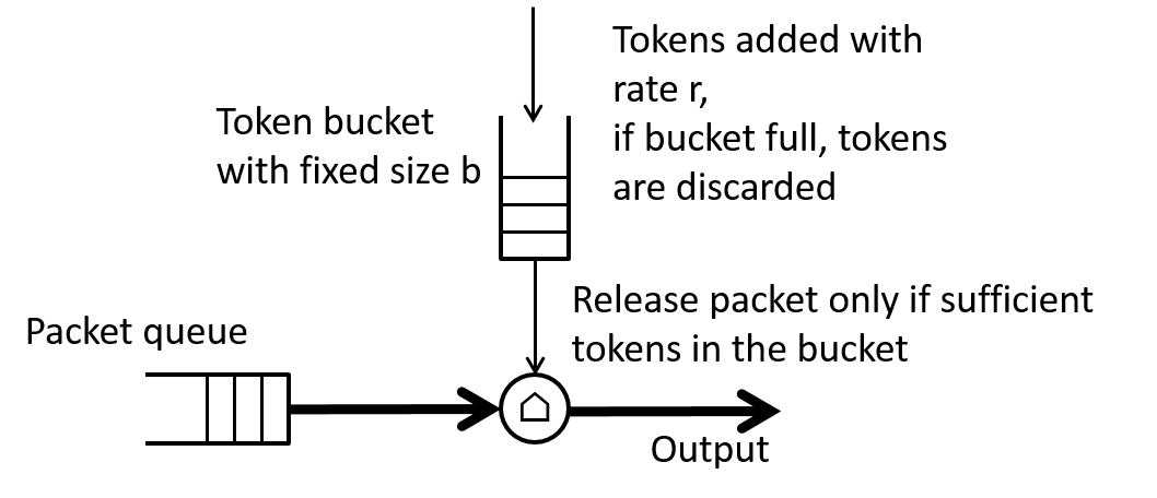
Figure 7. Basic token bucket traffic shaper.

At initialization the token bucket starts out full, i.e., with b tokens. Every $1/r$ time increment a token is added to the bucket. If the bucket is full then the extra tokens are discarded.

If a packet of size $L_p$ is at the head of the packet queue it will be transmitted only if the number of tokens in the bucket is greater than $L_p$. If that is the case then the packet will be transmitted and an equivalent of $L_p$ tokens will be "drained" from the bucket.

If there are less than $L_p$ tokens in the bucket then the packet will need to wait until enough tokens are added so that the number in the bucket is at least as large as $L_p$.

Traffic Shaper Behavior

Quiz:

What happens if I try to send a small bunch of back to back packets whose sum total length is less than the current bucket size?

Answer: All those packets will be burst out at the output line rate and we see that the maximum burst size at the line rate would be b.
What happens (limiting behavior) if I try to send a long stream of back to back packets through the shaper?

Answer: Very quickly (depending on b) the bucket will empty, and once it is empty each packet will need to wait $L_p/r$ for enough tokens to accumulate before it can be sent and hence packets will be sent with equivalent rate r.
What happens if I try to send a packet of length $L_p > b$ where b is the bucket size?

Answer: Since the length of the packet is greater than the number of tokens that can be put in the bucket the packet will never be transmitted. This is actually an configuration or implementation error. The minimum bucket size should always be greater than the maximum transfer unit (MTU).

Advanced Shaping and Implementations

Our basic shaper blasted out bursts of up to size b at the line rate. What if we wanted to further restrict the rate of these bursts to some peak rate $r_p$ which is less than the line rate, $r_{line}$, but greater than the average rate, $r_{avg}$? One way to implement this would be to add another token bucket shaper with rate $r_p$ and bucket size equivalent to one packet, i.e., an size of one MTU after an shaper with rate $r_{avg}$ as shown in Figure 8.

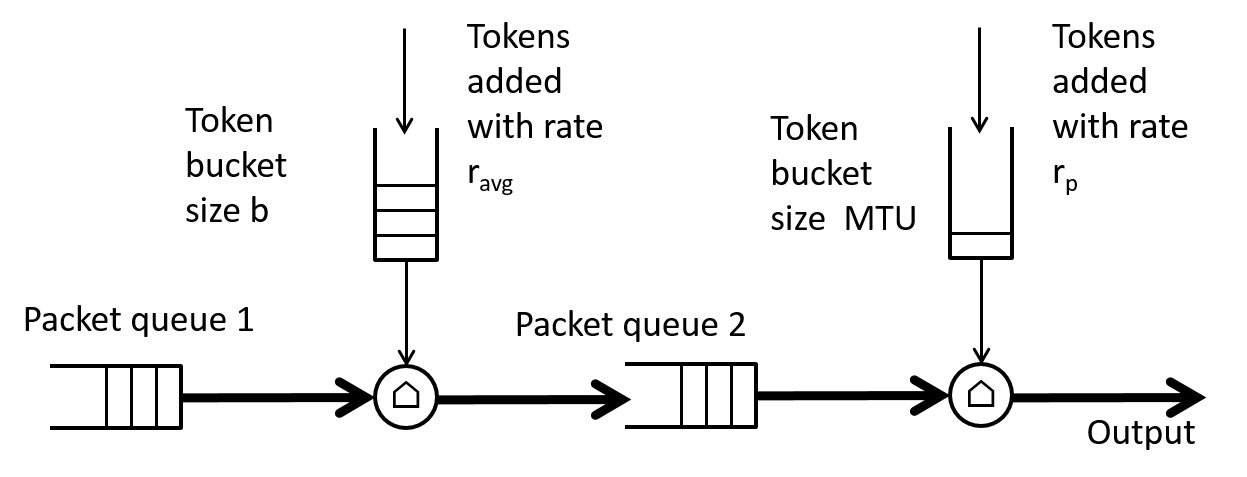
Figure 8. Average and peak rate shaping with two token buckets.

Note that $r_{avg} < r_p < r_{line}$.

You may be wondering where you can find such a traffic shaper in practice. At a Linux command line try typing man tc-tbf. On one of my Linux systems I get the following information:

NAME
       tbf - Token Bucket Filter

SYNOPSIS
       tc qdisc ... tbf rate rate burst bytes/cell ( latency ms | limit bytes ) [
       mpu bytes [ peakrate rate mtu bytes/cell ] ]

       burst is also known as buffer and maxburst. mtu is also known as minburst.

DESCRIPTION
       The Token Bucket Filter is a classful queueing  discipline  available  for
       traffic control with the tc(8) command.

       TBF  is a pure shaper and never schedules traffic. It is non-work-conserv‐
       ing and may throttle itself, although packets  are  available,  to  ensure
       that  the  configured  rate  is  not  exceeded.  It is able to shape up to
       1mbit/s of normal traffic with ideal minimal burstiness, sending out  data
       exactly at the configured rates.

       Much  higher  rates  are  possible  but  at the cost of losing the minimal
       burstiness. In that case, data is on average dequeued  at  the  configured
       rate  but  may  be  sent much faster at millisecond timescales. Because of
       further queues living in network adaptors, this is often not a problem.

ALGORITHM
       As the name implies, traffic is  filtered  based  on  the  expenditure  of
       tokens.   Tokens  roughly  correspond  to  bytes, with the additional con‐
       straint that each packet consumes some tokens, no matter how small it  is.
       This reflects the fact that even a zero-sized packet occupies the link for
       some time.

       On creation, the TBF is stocked with tokens which correspond to the amount
       of  traffic  that  can be burst in one go. Tokens arrive at a steady rate,
       until the bucket is full.

       If no tokens are available, packets are queued, up to a configured  limit.
       The  TBF  now  calculates the token deficit, and throttles until the first
       packet in the queue can be sent.

       If it is not acceptable to burst out packets at maximum speed, a  peakrate
       can  be  configured  to  limit the speed at which the bucket empties. This
       peakrate is implemented as a second TBF with a very small bucket, so  that
       it doesn't burst.

Traffic Shaper Simulation

We can gain additional insight into a token bucket traffic shaper by simulating one in Python via the SimPy library. Below we show the definition and constructor for our ShaperTokenBucket class. This models an ideal token bucket shaper. Note the token bucket size should be greater than the size of the largest packet that can occur on input. If this is not the case in our simulation we always allow the "bucket" accumulate enough tokens to let the current packet pass based on the average rate. This is slightly different from the behavior we previously defined.

The constructor takes the following parameters:

env : simpy.Environment; The simulation environment
rate : float; The token arrival rate in bits
b_size : Number; The token bucket size in bytes
peak : Number or None for infinite peak; The peak sending rate of the buffer (quickest time two packets could be sent)

class ShaperTokenBucket(object):
    def __init__(self, env, rate, b_size, peak=None, debug=False):
        self.store = simpy.Store(env)
        self.rate = rate
        self.env = env
        self.out = None
        self.packets_rec = 0
        self.packets_sent = 0
        self.b_size = b_size
        self.peak = peak

        self.current_bucket = b_size  # Current size of the bucket in bytes
        self.update_time = 0.0  # Last time the bucket was updated
        self.debug = debug
        self.busy = 0  # Used to track if a packet is currently being sent
        self.action = env.process(self.run())  # starts the run() method as a SimPy process

The implementation of the run and put methods for this class are shown below.

def run(self):
    while True:
        msg = (yield self.store.get())
        now = self.env.now
        #  Add tokens to bucket based on current time
        self.current_bucket = min(self.b_size, self.current_bucket + self.rate*(now-self.update_time)/8.0)
        self.update_time = now
        #  Check if there are enough tokens to allow packet to be sent
        #  If not we will wait to accumulate enough tokens to let this packet pass
        #  regardless of the bucket size.
        if msg.size > self.current_bucket:  # Need to wait for bucket to fill before sending
            yield self.env.timeout((msg.size - self.current_bucket)*8.0/self.rate)
            self.current_bucket = 0.0
            self.update_time = self.env.now
        else:
            self.current_bucket -= msg.size
            self.update_time = self.env.now
        # Send packet
        if not self.peak:  # Infinite peak rate
            self.out.put(msg)
        else:
            yield self.env.timeout(msg.size*8.0/self.peak)
            self.out.put(msg)
        self.packets_sent += 1
        if self.debug:
            print msg

def put(self, pkt):
    self.packets_rec += 1
    return self.store.put(pkt)

Note that this class is available in the SimComponents.py file that contains various discrete event simulation models for networking and is described in detail in the portion of the course on delay and blocking.

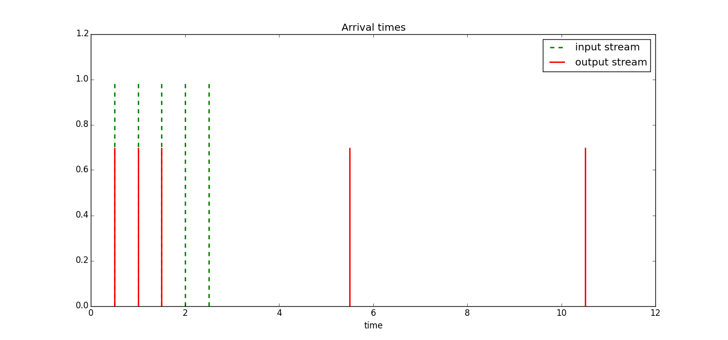
Example 1 Let's consider the case where we have burst of packets all with the same size with rate twice the bucket rate and where the bucket size is equal to the packet size. The simulation result is shown in Figure 9.

Figure 9. Shaper with input twice the rate and bucket size equal to one packet.

Note we don't see any bursts coming through since the bucket size is the same as the packet size. The ShaperExample1.py file contains the code used to produce Figure 9.

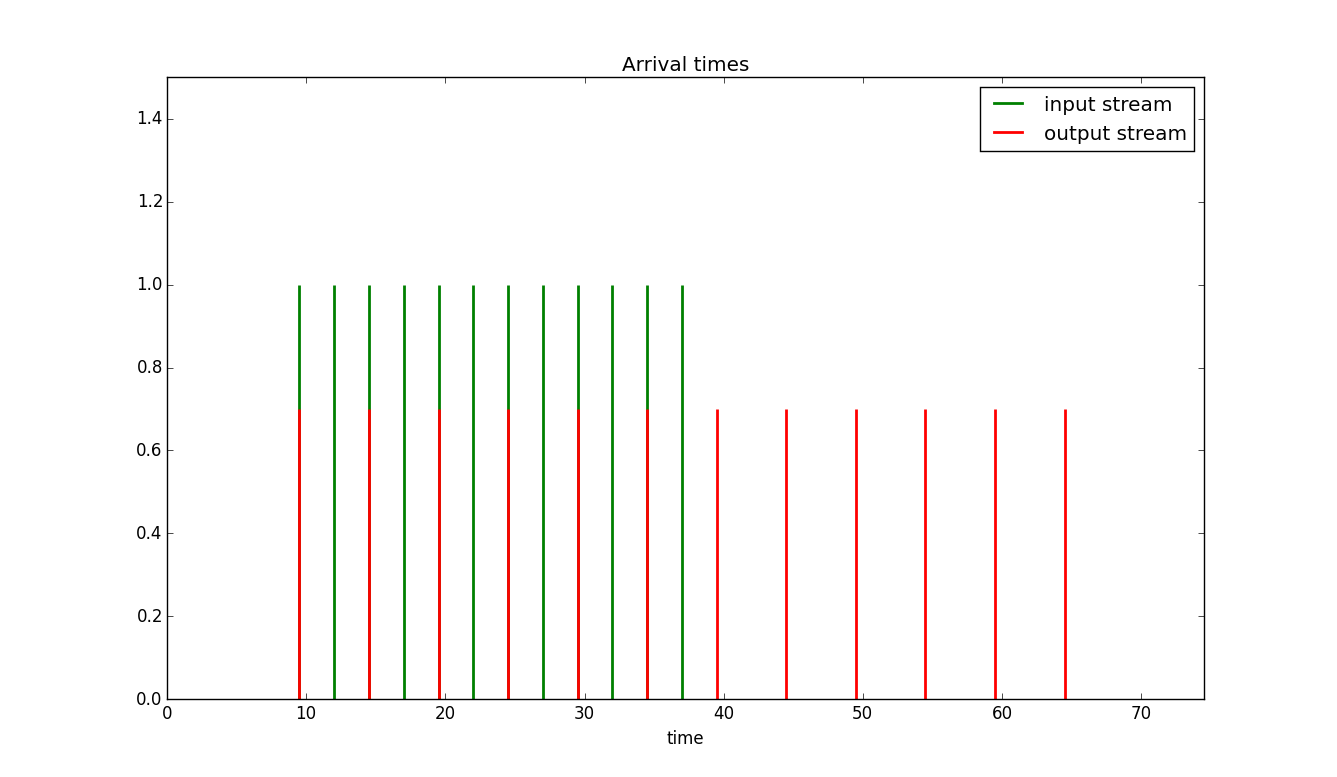
Example 2 Let's consider the case where we have burst of packets all with the same size with rate ten times the bucket rate and where the bucket size is equal to three times the packet size. The simulation result is shown below:

Figure 10. Shaper with input ten times the rate and bucket size equal to three packets.

In this case we clearly see the burst size parameter letting packets through that otherwise would need to wait a very long time. The ShaperExample2.py file contains the code used to produce Figure 10.

Poisson Arrivals through a Traffic Shaper

As might be expected for the case of Poisson traffic some analytic results are available concerning delays induced by the shaper. Here is one result from the analysis of reference [Bertsekas1992]. Let $L$ be the mean packet size in bits, $\lambda$ the packet arrival rate, $W$ the bucket size in bits, and $r$ the token rate. Let $\mu = r/L$ and $C = W/r$. Then the average delay is

$$E[D] = \frac{1}NaN{e^{ - C(\mu - \lambda )}}$$

Example: Let $\lambda = 0.5$ packets per second, $L = 125 \text{ bytes} = 1000 \text{ bits}$, $W= 10\cdot L=1250 \text{ bytes}$, $r = 625 \text{ bps}$, then $\mu = 0.625$, and $C = 16 seconds$ which gives $E[D] = 1.082682$. You can simulate this result via SimPy, the ShaperTokenBucket class as shown in the file ShaperExampleRandom.py.

Is there anything that seems odd with this result or the simulation? Recall that we said that if the packet size was larger than the bucket size then no packets would ever be sent and using a exponential distribution for the packet size there is always a chance of the packet size exceeding the bucket size. So under what conditions did reference [Bertsekas1992] derive this result? They assumed that if the packet size exceeds the bucket size then the packet will be fragmented into multiple pieces with the size of each piece being less than or equal to the bucket size. This is similar to IP fragmentation or TCP using segments less than the MTU size to avoid IP fragmentation. In our shaper simulation code we let enough tokens build to release a packet of any given size. To more accurately model the real world we'd need to modify our packet sources to do fragmentation (Sometimes a homework assignment in this class).

Flow Characterization and Policing

We saw earlier that if we can bound the behavior (rate) of a source than we can obtain bounds on delays and make guarantees on packet loss given sufficient buffer sizes. We then saw that a shaper can be used to make sure a traffic flow conforms to a given set of bounds. The price for this was the introduction of (controlled) delays into the packet stream. Since a network user frequently judges a network based on the delays its packets encounters, networks typically want to minimize operations such as shaping that add delays. Instead the network will offer guarantees on delays and packet loss to traffic that meets particular bounding constraints. Hence network users perform shaping on their traffic prior to it entering a network.

To establish that the user's traffic actually corresponds to the bounds that they promised to meet the network performs traffic policing. A policer is a logical network element that will either mark or drop non-conforming packets in a flow.

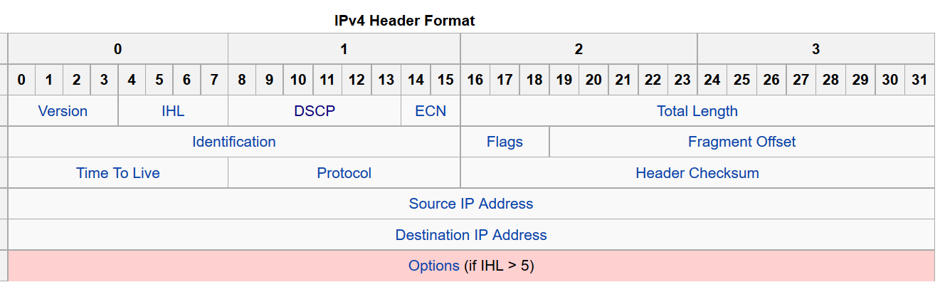
Since droping a packet can be considered a rather extreme form of policing the option of marking a non-conforming packet is frequently more desirable. In fact current IP standards support three levels of marking. In Figure 11 we show a fairly up to date diagram of the IPv4 packet header. Byte 1 (not 0) contains the 6 bit differentiated services code point (DSCP) and the 2 bit explicit congestion notification (ECN) fields. For conformance marking we will only be concerned with the DSCP bits.

Figure 11. IPv4 packet header from Wikipedia. Note in byte 1 the DSCP and ECN fields.

RFC2597 provides a specific example of using the DSCP field to support four service classes (whose QoS guarantees would be defined by the network carrier) along with three markings for packet loss precedence, i.e., which packets would get dropped first. We show the recommended assignments in the Figure 12. In Figure 12 the left most 3 bits are used to define the class while the next 2 bits are used to set the drop precedence. It is important to note that IP routers are allowed to modify the bits in the DSCP field and the logical policing element will typically reside within a router.

Figure 12. Use of the DSCP field in the IPv4 header to provide classes of service and drop precedence.

Now all we need to figure out is how to implement a traffic policer. It turns out that we can just use token bucket techniques in a slightly different way than they were used for traffic shaping. We will look at two different policers specifically designed for IP traffic.

A Single Rate Three Color Marker

A policer called a single rate three color marker (srTCM) is defined in RFC2697 an informational RFC. The single rate means we will use a single token generator with a specified rate parameter. By three color they mean that packets will be marked with by three levels of compliance (Green, Yellow, Red) from compliant to most out of compliance.

This particular policer is defined by three traffic parameters, an update algorithm, and marking criteria. The three traffic parameters are:

Committed Information Rate (CIR) measured in bytes of IP packets per second, i.e., it includes the IP header, but not link specific headers. This is the token rate.
Committed Burst Size (CBS) measured in bytes. This is the token bucket size associated with the rate.
Excess Burst Size (EBS) measured in bytes. This is a bucket filled from the overflow of the first bucket hence the expression "excesses burst size". This bucket allows us to save up tokens from periods of inactivity for later use. The CBS and EBS must be configured so that at least one of them is larger than 0.

There are two modes of operation for the srTCM one, called Color-Aware works with packets that have been previously marked by another policer in the network, the other mode called Color-Blind works with packets that have not been previously marked. The Color-Blind mode of operation is shown in Figure 13.

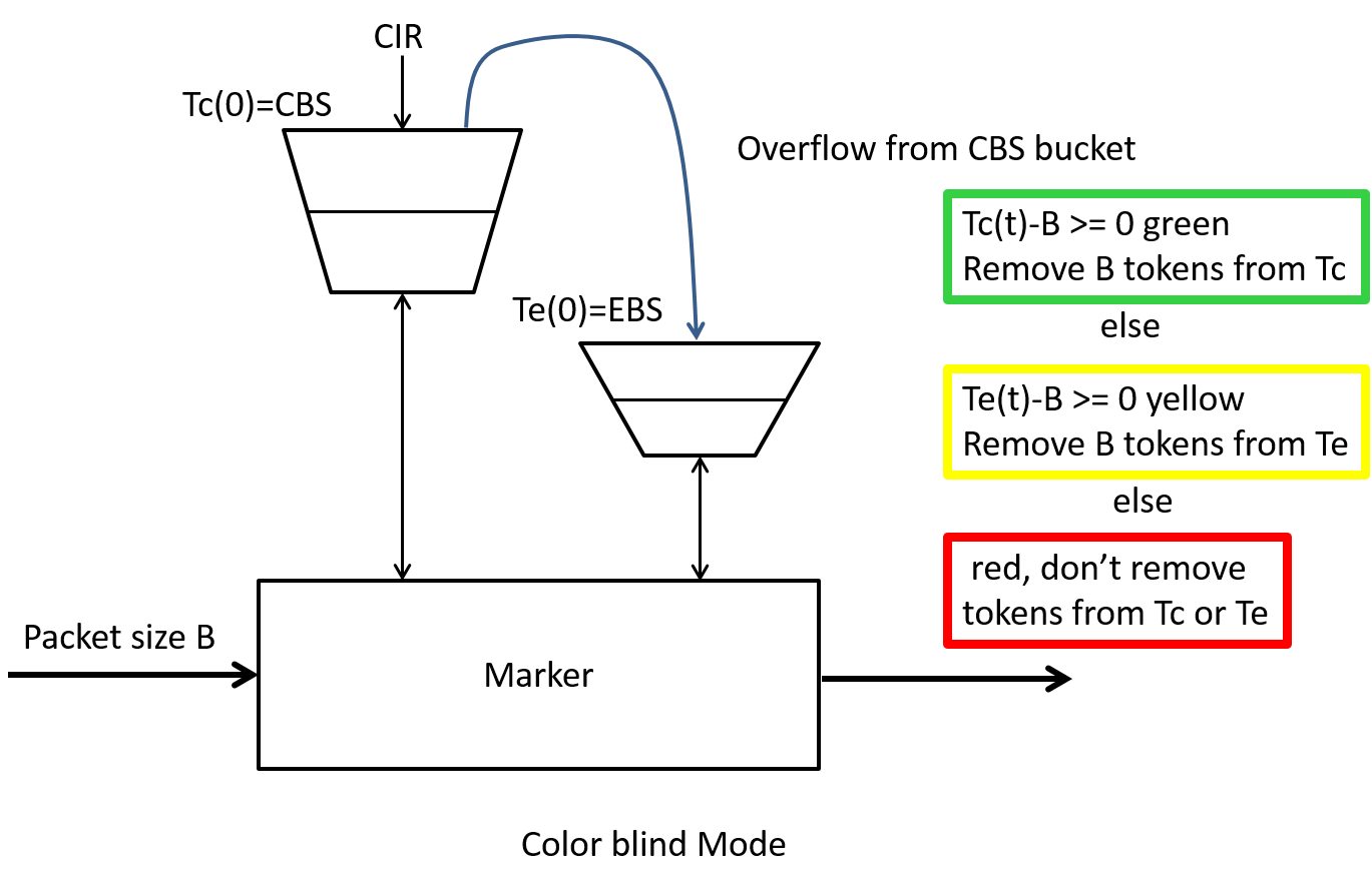
Figure 13. Single rate, three color marker.

Initialization and Update

The two token buckets are represented by the token count state variables $T_c(t)$ and $T_e(t)$ respectively. At time $t=0$, $T_c(0) = CBS$ and $T_e(0) = EBS$, i.e., both buckets start full. These variables are updated every CIR times per second as follows:

If $T_c$ is less than CBS, $T_c$ is incremented by one (this corresponds to one byte of IP packet), else
if $T_e$ is less then EBS, $T_e$ is incremented by one, else
neither $T_c$ nor $T_e$ is incremented.

Basically we fill the first bucket with tokens, excess tokens can fill the second bucket and once its full we just throw away the tokens.

Packet arrival and Marking When a packet of size B bytes arrives at time t, the following update and marking takes place:

If $T_c(t)-B \geq 0$, the packet is marked green and $T_c$ is decremented by B down to the minimum value of 0, else
if $T_e(t)-B \geq 0$, the packets is marked yellow and Te is decremented by B down to the minimum value of 0 (here we are looking at tokens we may have saved up in the excess bucket), else
the packet is marked red and neither $T_c$ nor $T_e$ is decremented. (This is the case where we are have insufficient tokens in either bucket)

You may get to try some packet marking examples with the srTCM in the homework. Note that if EBS is set to zero then we have a simple green/red test for conformance with our previous theoretical $(\sigma,\rho)$ traffic bound.

Two rate three color marker

Another policer called a two rate three color marker (trTCM) is defined in RFC2698, an informational RFC. The two rate means we will use a two token generators each with a specified rate parameter. Once again the three colors Green, Yellow, Red indicate the level of compliance which gets translated into packet drop precedence when the packets get marked. The parameters for this policer are: the Peak Information Rate (PIR), the Peak Burst Size (PBS), the Committed Information Rate (CIR), and the Committed Burst Size (CBS). All use units similar to that of the srTCM. The initialization, update, and marking behavior for the Color-Blind mode is shown Figure 14.

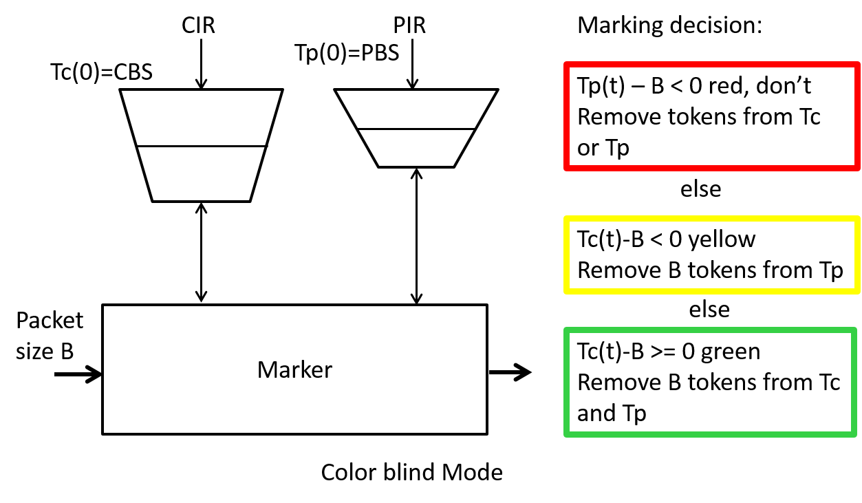
To understand if this policer will mark packets as we expect lets look at some example cases.

Case 1: Stream of packets at a rate above the PIR

We'll assume that PBS is less than CBS. Both buckets start full so initially any packets coming in will be marked green and both buckets will be decremented. However since the packets are coming in faster than PIR we will drain both buckets and eventually the peak bucket will be drained empty so that packets will be marked red. While this is happening both buckets will get to fill again. When the peak bucket is full enough packets will get to be marked either green or yellow however the draining of the peak bucket will resume and we will see packets marked red again. This process will continue to repeat itself.

Case 2: Stream of packets at a rate above the CIR but below the PIR

In this case the peak bucket which starts full will never drain to the point where packets get marked red. However with each green marked packet the CIR bucket will drain faster than it can fill until we start having to mark packets yellow. When we mark packets yellow we aren't removing tokens from the CIR bucket so it will fill again enough so that we mark some packets green then it will drain and packets will be marked yellow. Hence in this case we will see a stream of packets marked either green or yellow.

Case 3: Stream of packets at a rate below the CIR

In this case, since the buckets start full and the packet rate is less than the CIR, none of the buckets will drain to the point where the bucket count is less than the packet size. Hence all packets will be marked green.

Simulating Policers/Markers

Creating simulation models of the single rate three color marker and the two rate three color markers previously defined were given as homework problems in class. If readers are interested in seeing some examples send me an email and I'll update this section.

Policing in Linux

Linux traffic control provides for policing though information is very difficult to find in the Linux man pages. One of the best sources of information is the Linux documentation project's traffic control How-To or the Linux advance routing and traffic control website particularly their section on advanced filtering and policing. Linux's policer is a single bucket (rate and burst size) two color (green or red) implementation by combining these in clever ways the documentation claims one can create a three color marker but I couldn't find any clear examples to point you towards :-(.

A system that uses Linux traffic control (tc) policing indirectly is the policing feature of Open vSwitch. See this page for a simple example.

Packet Scheduling

We've seen how to shape and police flows to nice predictable bounds. However much of the time in packet switching senders may be well under their average rate bounds. In such a case, there should be lots of idle bandwidth available on a link. How can we allow this bandwidth to be used while still maintaining guaranteed bandwidth for users who have paid for it? In this case think of an enterprise utilizing "private line" Ethernet or MPLS services. Or suppose that there are no bandwidth guarantees and all service is "best effort", how can we distribute the available bandwidth fairly amongst users?

Packet scheduling, which decides when and which packets get sent on a port, will help us make good use of link bandwidth. Modern packet scheduling techniques can offer: (a) protection from badly behaved users, (b) better than worst-case guarantees for delay and loss, (c) better sharing of unused bandwidth, (d) separate delay and bandwidth guarantees. A very good overview of packet scheduling for guaranteed service is reference [HZhang1995].

Fairness and Packet Scheduling

The first queueing disciplines we will look at works in best effort situations to insure fairness amongst users.

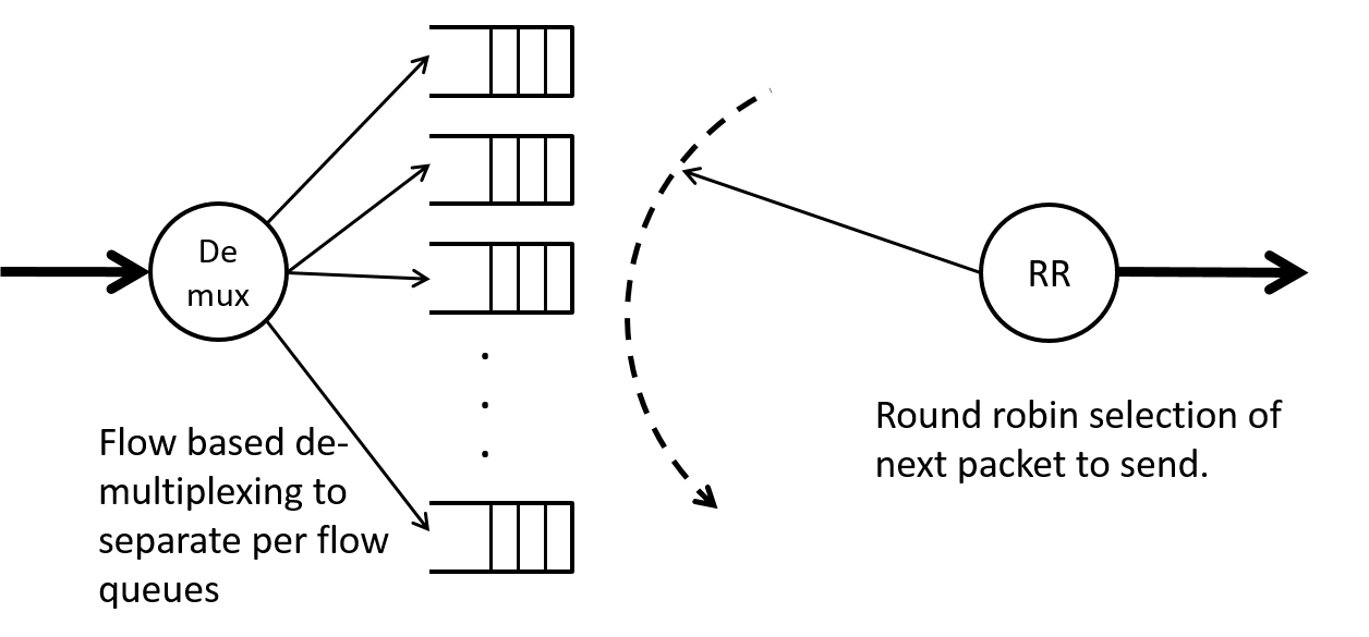
Round Robin

One way to assure fairness to different flows is to give each flow its own queue and then “serve” each queue in some predefined order that rotates evenly over all queues. Such an approach is known as Round Robin and is commonly used in many areas of computer science as well as networking and in other parts of life. A diagram of round robin scheduling applied to packet flow is shown in Figure 15.

Stochastic Fairness Queueing

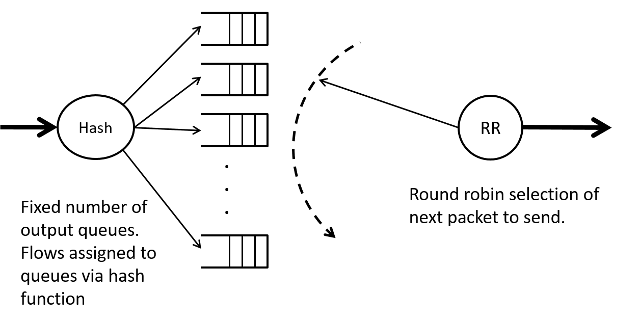
The problem with the previous flow based round robin is that we'd need to classify packets into separate flows and then set up separate queues for each flow, then determine the order to serve the flows, and iterate the service amongst all these queues. Since there can be a potentially great number of flows this presents implementation challenges.

A very sucessful and widely adopted alternate approach was suggested by McKenny in 1990 [McKenney1990] and is called Stochastic Fairness Queueing (SFQ). To limit the number of queues that need to be served via a round robin scheduler to a reasonably small number SFQ assigns flows to queues via a hash function as shown in Figure 16. To avoid the unfairness of a well behaved user being “binned” with a badly behaved user one can periodically change the hash function.

Figure 16. Stochastic Fairness Queueing.

SFQ is available in most Linux distributions via Linux traffic control tc. Below is a portion of the man page (man tc-sfq). It should be noted that simply changing the hash function without paying attention to the queues can result in packet re-ordering within a flow which is generally bad for performance for protocols such as TCP. This is pointed out in the man page and has been fixed in newer Linux kernel releases.

NAME
       sfq - Stochastic Fairness Queueing

SYNOPSIS
       tc  qdisc  ...   [  divisor hashtablesize ] [ limit packets ] [ perturb
       seconds ] [ quantum bytes ] [ flows number ] [ depth number ]  [  head‐
       drop ] [ redflowlimit bytes ] [ min bytes ] [ max bytes ] [ avpkt bytes
       ] [ burst packets ] [ probability P ] [ ecn ] [ harddrop ]

DESCRIPTION
       Stochastic Fairness Queueing is a classless queueing discipline  avail‐
       able for traffic control with the tc(8) command.

       SFQ does not shape traffic but only schedules the transmission of pack‐
       ets, based on 'flows'.  The goal is to ensure  fairness  so  that  each
       flow is able to send data in turn, thus preventing any single flow from
       drowning out the rest.

       This may in fact have some effect in mitigating  a  Denial  of  Service
       attempt.

       SFQ is work-conserving and therefore always delivers a packet if it has
       one available.

ALGORITHM
       On enqueueing, each packet is assigned to a hash bucket, based  on  the
       packets  hash value.  This hash value is either obtained from an exter‐
       nal flow classifier (use tc filter to set them), or a default  internal
       classifier if no external classifier has been configured.

       When the internal classifier is used, sfq uses

       (i)    Source address

       (ii)   Destination address

       (iii)  Source and Destination port

Bandwidth Guarantees and Allocation

We will look in depth at one of the first modern queueing disciplines that provided explicit bandwidth guarantees known as Virtual Clock [LZhang1990]. We then will look at enhancements offered by Generalized Processor Sharing [Parekh1993] queueing discipline.

Virtual Clock Goals and Benefits [LZhang1990]:

Keeps the benefits of statistical multiplexing
Controls average transmission rate of flows
Enforce each user’s resource usage
Build firewalls between the flows (don’t let badly behaved users hurt the QoS of well behaved users).

Inspired by TDM systems, we assign an average bandwidth to each flow and make sure that the sum of those bandwidths does not exceed the line rate. However we want to stay work conserving, so instead of assigning each packet a “transmission slot” instead we will appropriately order packets for transmission.

Understanding Virtual Clock

"Hey kids, what time is it?" "Its time to send a packet for flow j!"

The above quote from a non-existant childrens television program gives us a hint at what the virtual clock packet scheduler is all about. We are interested in guaranteeing flow j, $r_j$ units of bandwidth. Here $j=1 ... N$, where $N$ is the number of flows. We assume the line rate on our switch port is C and that $C < \sum_j r_j$.

In analogy with TDM let's imagine that each flow j gets its own $r_j$ bandwidth link. What would be the transmission (send) time for the first packet from flow j? It would simply be the arrival time plus the time it would take to send the packet at rate $r_j$:

$$Tsend_j^1 = TArrival_j^1 + \frac{L_j^1}{r_j} \tag{VC1}$$

where $Tarrival_j^k$ is the time of arrival of the k^th^ packet from flow j and $L_j^k$ is the length of the k^th^ packet in bits from flow j. If we define a virtual clock tick time for flow j by $$Vtick_j = \frac{1}{r_j}$$

Then our previous sending time equation (VC1) becomes:

$$Tsend_j^1 = TArrival_j^1 + Vtick_j \cdot L_j^1$$

Now we need to figure out when the next packet from j would be send, i.e., $Tsend_j^2$. Note that we are not using superscripts to denote taking a quantity to a power in this notation! There are some basic rules that need to be obeyed:

The second packet from flow j can't start to be transmitted until after the first packet finishes. If the second packet arrives while the first packet is being virtually sent we would get the following $$Tsend_j^2 = Tsend_j^1 + Vtick_j \cdot L_j^2 \tag{VCF2a}$$
In accordance with the laws of reality (causality to be specific) the second packet can't be sent before it arrives. Hence if the second packet arrives after the first packet has been completely sent we would have: $$Tsend_j^2 = Tarrival_J^2 + Vtick_j \cdot L_j^2 \tag{VCF2b}$$

If we want to compactly specify both these rules, equations (VCF2a) and (VCF2b) we can write: $$Tsend_j^2 = \max(Tarrival_j^2,Tsend_j^1) + Vtick_j \cdot L_j^2$$

Now generalizing this to the sending time of the k^th^ packet gives us: $$Tsend_j^k = \max(Tarrival_j^k,Tsend_j^{k-1}) + Vtick_j \cdot L_j^k \tag{VCUpdate}$$

You maybe thinking "how does this help us with a real switch port"? The method is to use the "virtual" sending time derived above as a piece of information, a virtual clock timestamp, that we'd associate with a packet. We then sort packets in the output queue by these virtual timestamps, choosing the packet with the lowest timestamp to be sent next.

The notation frequently seen in the literature uses $a_j^k$ as the arrival time of the k^th^ packet from flow j and $auxVC_j^k$ as the virtual sending time leading to the slightly shorter but more cryptic expression:

$$auxVC_j^k = \max(a_j^k,auxVC_j^{k-1}) + Vtick_j \cdot L_j^k$$

Now lets look at some properties of the $auxVC_j$ timestamps to help us understand how they provide bandwidth guarantees and isolation between flows.

Time stamps can never fall behind real time. This implies there is no reason not to send packets, i.e., one can't build up "credit" to be used later.
If source j sends packets with an average rate less than $r_j$ then the virtual timestamps $auxVC_j^k \approx a_j^k +L_j^k \cdot Vtick_j$ most of the time. With priority based on the timestamps this means that it does look to flow j that it has its own $r_j$ bandwidth channel.
If flow i sends at an average rate much greater than $r_i$ then its $auxVC_i^k$ timestamps will build up to be much greater than the real time and hence packets from flow i will tend to be sent after packets from a "conforming" flow j. This is how virtual clock packet scheduling provides isolation betweeen different flows, i.e., protection from badly behaving flows.

Simulating Virtual Clock

Now lets look at how we would simulate an output port featuring virtual clock based scheduling. In the code below we show our VirtualClockServer class. It is initialized with the line rate and an array of vtick values, one for each flow that will exit the output port. We keep an array of the current auxVC values in the list self.auxVCs.

The auxVC value for a particular flow is updated in the put function when a new packet comes in. This packet along with its virtual clock timestamp gets put in our special StampedStore priority queue (implemented via a python heap but not shown). The run code looks the same as the FIFO queue that we used when simulating queueing systems, but in this case the StampedStore queue always returns the packet with the lowest timestamp.

class VirtualClockServer(object):
    def __init__(self, env, rate, vticks, debug=False):
        self.env = env
        self.rate = rate
        self.vticks = vticks
        self.auxVCs = [0.0 for i in range(len(vticks))]  # Initialize all the auxVC variables
        self.out = None
        self.packets_rec = 0
        self.packets_drop = 0
        self.debug = debug
        self.store = StampedStore(env)
        self.action = env.process(self.run())  # starts the run() method as a SimPy process

    def run(self):
        while True:
            msg = (yield self.store.get())
            yield self.env.timeout(msg.size*8.0/self.rate)
            self.out.put(msg)

    def put(self, pkt):
        self.packets_rec += 1
        now = self.env.now
        flow_id = pkt.flow_id
        self.auxVCs[flow_id] = max(now, self.auxVCs[flow_id]) + self.vticks[flow_id]*pkt.size*8.0
        return self.store.put((self.auxVCs[flow_id], pkt))

Note that the complete code for this Python class is contained in the SimComponents.py file.

Example 1 Suppose with have a link with a line rate of 992Mbps, and we have two sources each sending packets of size $L=100\text{ bytes}$. We allocate 320Mbps to each source, i.e., $r_j =1/Vtick_j=320\text{ Mbps}$ Now suppose that source 0 sends a set of packets at a constant rate of 320Mbps and source 1 sends a set of packets at 3.2Gbps (10 times its allocation). In the top half of Figure 17 we show the arrival rate times of the packets from source 0 in green and source 1 in red. The sending rate difference between the sources is very clear here. In the second half of Figure 17 we show the departure times from the switch port. We see that source 0's packets incur minimal delay (a micro second or so) while source 1's packets incur significant delay, i.e., look at the spread in time from when the last packet of the bunch arrived (at around $15\mu s$) til when it finally leaves (at around $45\mu s$).

Note also that even though source 1 was badly behaved it was still allowed to use the remaining spare capacity on the link rather than being restricted to a fixed 320Mbps allocation. This is because virtual clock is a work conserving scheduling mechanism and will always send packets if there is available capacity. Contrast this with a packet shaper who's job it is to restrict the flow. A shaper is not work conserving.

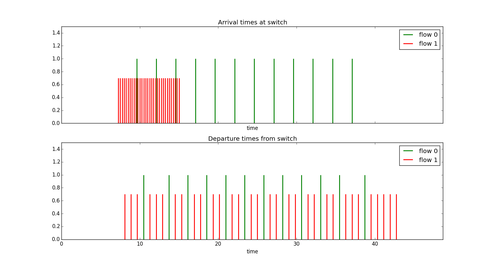
Figure 17. Virtual clock example with a "good" source and a "bad" source.

Note that the only reason that we use a constant packet size is that it gives us easy to interpret simulation plots, if the packet size varied then even for a source sending at a constant rate the send times would vary.

Example 2 In this simulation we have two well behaved sources and two somewhat badly behaving sources. Once again all packets will be a constant size of 100 bytes. We will assume a line rate of 8 Mbps. The sources allocations and sending rates are:

Source #0 is allocated 1.5 Mbps and sends at 1.25 Mbps (good)
Source #1 is allocated 2.0 Mbps and sends at 4.0 Mbps (bad)
Source #2 is allocated 2.5 Mbps and sends at 2.0 Mbps (good)
Source #3 is allocated 1.25 Mbps and sends at 4.5 Mbps (even more bad)

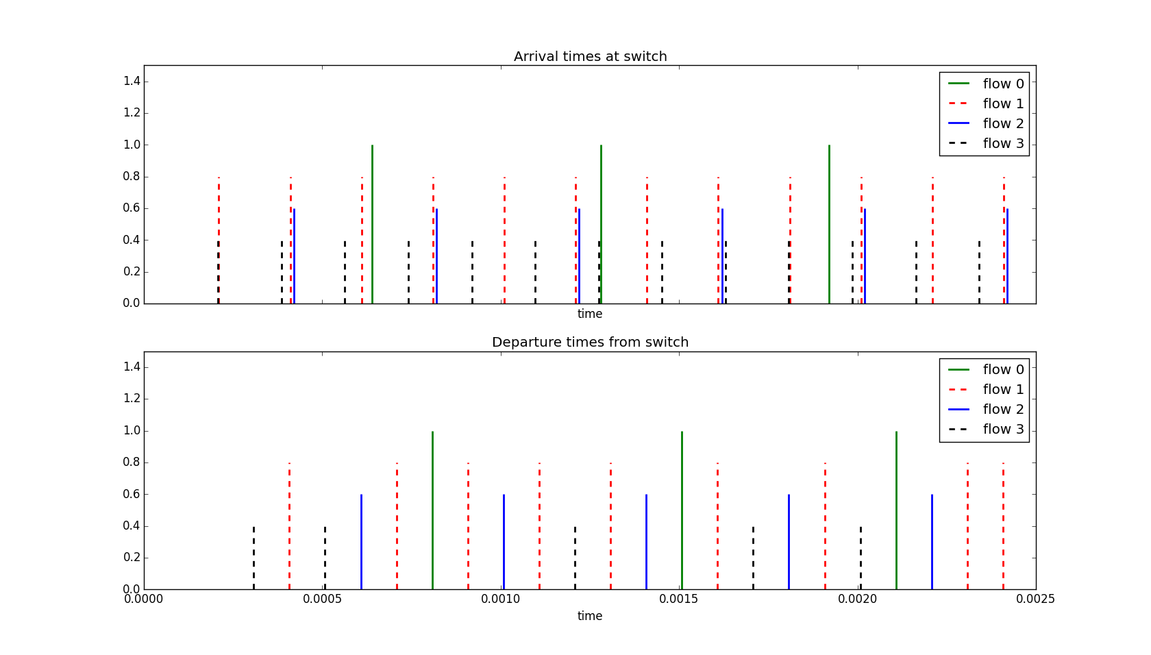
Figure 18. Virtual clock example with multiple "good" and "bad" sources.

Can you see how the packets from source 1 (one of our bad sources) get slowed down. For source 3 (and even more badly behaving sources) which starts early before the output link gets busy we see that its first two packets incur minimal delay but the next incur significant delay in line with its lower allocated rate.

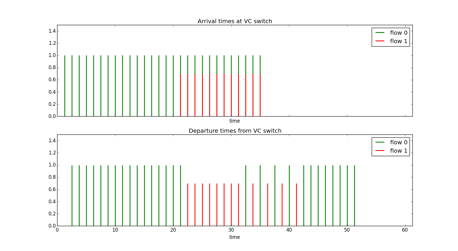
Example 3 Two sources each allocated half the line bandwidth and each transmitting at the line rate with one starting before the other. In the top half of Figure 19 we see the arrival times of packets from the two sources. Source 0 starts first then later Source 1 starts. We see that when source 1 starts sending for a while it gets to dominate the output port until its virtual clock catches up to source 0's and then they share the link evenly. In a sense source 0 was punished for exceeding its average rate even though no other sources were using the link at the time.

Figure 19. Virtual clock example with two over rate sources.

An issue that we saw in our last simulation of virtual clock is that it punishes users for using more than their allocation of the link bandwidth even when the link is under utilized. This is a problem since we want users to make more efficient use of network links which means we want to encourage them to use more bandwidth during times when the link isn't full.

A packet scheduling scheme that goes by either the name of Weighted Fair Queueing (WFQ) [HZhang1995] or Generalized Processor Sharing (GPS) [Parekh1993] keep the nice properties of Virtual Clock and eliminates this drawback. The scheme uses a time stamp like Virtual Clock but has a different method for updating the time stamps.

In WFQ/GPS the timestamp is called a virtual finishing time and the virtual finishing time for the k^th^ packet of the i^th^ flow is denoted by $F_j^k$. To avoid punishing users for using more than their allocation we will work with a virtual time variable, $V(t)$ where t is the real time, that will be shared by all flows. We will then do the following:

At any time t when the output link is not busy (system is empty) we set $V(t) = 0$ and we reinitialize all the $F_j^k = 0$.
Whenever the server is busy we track all arrival and departure events, between the (k-1) event and the k event we set the virtual time as follows $$V(t_{k-1} + \tau) = V(t_{k-1}) + \frac{\tau}{\sum_{i \in B_k}\phi_i}$$ where $B_k$ is the set of currently active flows (and not all the flows), and the $\phi_j$ is the rate allocation for flow j (the equivalent of the $r_j$ in Virtual Clock), and $0 \le \tau \le t_k - t_{k-1}$.

Now when we go to update the virtual finishing times we use this virtual time rather than the raw arrival time: $$F_j^k = \max(F_j^{k-1}, V(a_j^k)) + \frac{L_j^k}{\phi_j}$$

Notes: The odd updating of the virtual time results in bandwidth sharing proportional to the active flows rate allocation. The reseting of the virtual time and timestamp variables to zero when the server isn't busy prevents users from being punished for using more than their allocation during non-busy times.

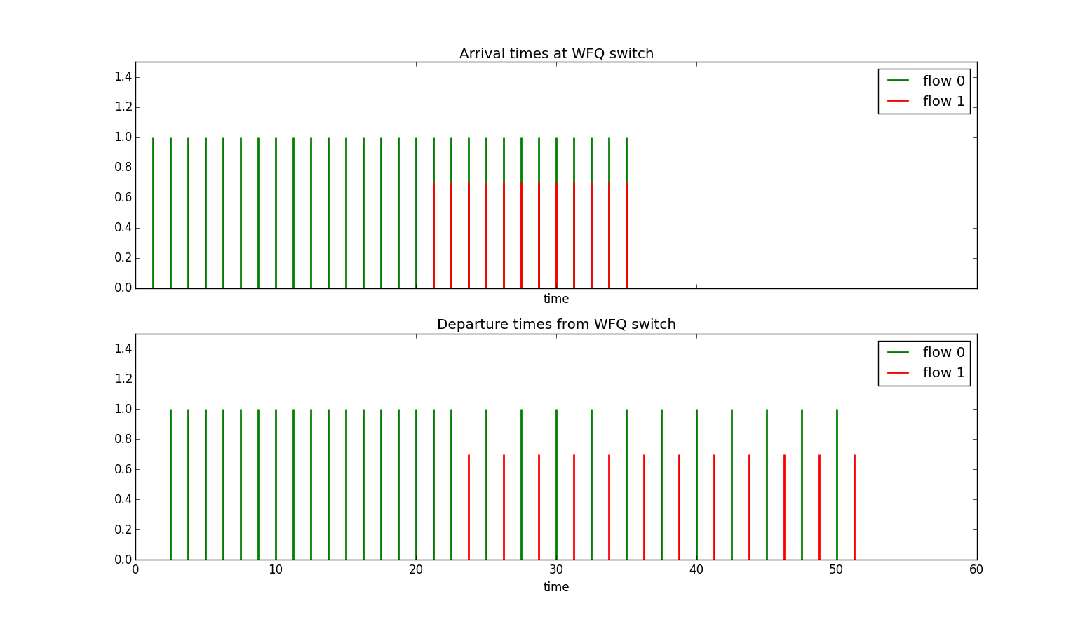
Example Let's revisit the last Virtual Clock example but this time with a WFQ server. In that example we had two sources each allocated half the line bandwidth and each transmitting at the line rate with one starting before the other. In the top half of the figure below we see the arrival times of packets from the two sources. Source 0 starts first then later Source 1 starts. In this case although source 0 was transmitting above its allocated rate it wasn't penalized for this when source 1 started sending its packets. When both sources 0 and 1 are sending the bandwidth is evenly divided between them. Note however if source 0 had been sending above the line rate and built up a queue those queued packets would have to share with other sources during the busy period.

Figure 20. WFQ/GPS example with two sources both sending above their allocations.

Delay, Jitter, and Queue Bounds for VC/WFQ/GPS

We saw that both Virtual Clock and WFQ/GPS provide bandwidth guarantees to flows and isolation from badly behaving flows. However, they both can be shown to give better bounds on delay, jitter, and queue sizes than those we previously studied.

Let source j be $({\sigma_j}, {\rho_j})$ bounded, $L_{\max }$ be the maximum packet size in bits, assume the $i^{th}$ switch encountered by flow j has output speed $C_i$ and that flow j has been allocated rate $r_j$. For the Virtual Clock and WFQ/GPS queueing disciplines the following bounds can be derived [HZhang1995]:

End to End Delay Bound

$$\frac{\sigma_j + nL_{\max }}{r_j} + \sum\limits_{i = 1}^n {\frac{L_{\max}}{C_i}}$$

End to End Jitter Bound

Here we define jitter as the maximum difference in the delays of any two packets [HZhang1995].

$$\frac{\sigma_j + nL_{\max}}{r_j}$$

Buffer space needed at the hth switch for flow j

$$\sigma_j + hL_{\max }$$

HFSC: Hierarchical Allocation, Separate Bandwidth & Delay Guarantees

The most advanced packet scheduling technique we will look at is called Hierarchical Fair Service Curve (HFSC) [Stoica2000]. This scheduling algorithm provides bandwidth guarantees and hard bounds on delay like Virtual Clock and WFQ, and provides "fair" link sharing like WFQ without the "punishment" we saw with virtual clock for users that used excess bandwidth (without building up a queue). HFSC adds in two important additional features: hierarchical bandwidth allocation, and separate bandwidth and delay bounds.

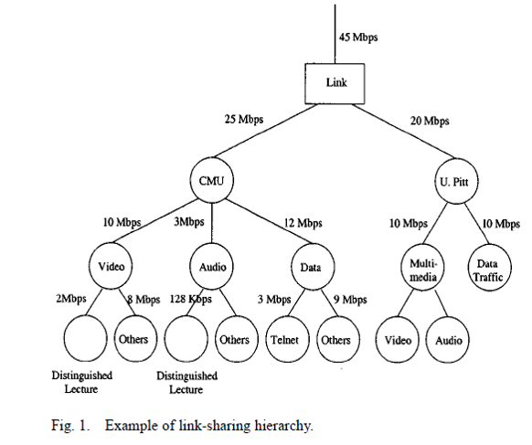
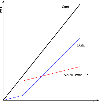
In Figure 21, from [Stoica2000], we show what we mean by hierarchical bandwidth allocation. Here a 45Mbps WAN link is being shared by two universities CMU and University of Pittsburg (U. Pitt). CMU is allocated 25Mbps of the bandwidth and U. Pitt 20Mbps. Within those two institutions the bandwidth is further divided into service classes such as video, audio, data, etc. that get allocated a share of the bandwidth allocated to the institutions, i.e., a bandwidth allocation hierarchy. At the very bottom of the hierarchy we may see leaf nodes that have particular "hard" or "realtime" requirements for bandwidth or latency such as video, audio, or file transfer. The challenge that HFSC overcomes is to allow sharing of unused bandwidth in conjunction with the bandwidth allocations given in the hierarchy in a way that is reasonably fair and that is guaranteed to meet the bounds required by the leaf nodes (like Virtual Clock and WFQ). We say "reasonably" fair since [Stoica2000] shows that it is impossible to be perfectly fair at all times in all situations.

Figure 21. Example of hierarchical bandwidth allocation from Stoica2000.

HFSC allows for somewhat separate specification of delay and bandwidth bounds. Consider a packet of length L arriving at a busy WFQ based output port. The packet will be stamped with a virtual finish time equal to $L/r$ where $r$ was the flows allocated WFQ rate. This could happen at each switch the packet encounters and hence led to the delay bounds we saw at the end of the previous section. Note that this delay bound is dependent on the allocated rate $r$. Now suppose we have a low rate delay sensitive service such as VoIP. The analysis given next is based on an HFSC in Linux blogpost. Suppose that VoIP requires 100kbps of bandwidth, and uses 1500 byte packets then under our worst case scenario each busy output port could add $(8 \text{ bits/byte} \cdot 1500 \text{ bytes})/100 \text(kbps) = 120 \text{ mS}$ of delay to this stream which would quickly result in unacceptable service.

Although we could up the allocated rate to reduce the delay this then leads to suboptimal bandwidth allocation and sharing. HFSC resolves the tight link between delay bounds and bandwidth with the idea of a service curve. A service curve in HFSC is a function of time that indicates how much service (in bits or bytes) a flow receives over a particular time period (this time period is related to the flows busy period). In Figure 22 we show two service curves from the HFSC blogpost. The red curve in Figure 22 shows a recommended service curve for VoIP. Since the horizontal axis is time and the vertical axis is bits the slope at any point of the service curve is an instantaneous rate. In the VoIP curve they gave the first segment of the curve a rate of 400kbps, the second slope of the curve a rate of 100kbps (the average rate VoIP rate) and the breakpoint occuring at 30mS of time. Intuitively this will have the effect of reducing the worse case delay that could be incurred by 3/4. Note for rigorous proofs you need to consult [Stoica2000]. Such benefit doesn't come for free. If $S_i(t)$ is the service curve of the i^th^ flow then [Stoica2000] states that the guarantees can only be achieved if $\sum_i S_i(t) \leq S(t)$ for all $t \ge 0$ where $S(t)$ is the service curve of the output link (just a straight line through the origin with slope equal to the line rate). In the figure below they achieve this by slowing down the initial rate that the "data" flow would receive.

Figure 22. HFSC service curves and their sum.

We've just scratched the surface of the HFSC scheduling algorithm. HFSC is important not only due to its very complete set of capabilities but also due to its wide availability via Linux. However, good information on HFSC can be hard to find I recommend (for now) the following:

The original HFSC journal paper [Stoica2000]. There was an earlier conference paper but this version is a bit clearer.
The web page HFSC Scheduling with Linux
A HFSC tutorial on sourceforge

There is a similar sounding Linux packet scheduler called Hierarchical Token Bucket (HTB). Although this seems to be popular there doesn't seem to be any rigorous analysis available. Note in his theory section he does cite a paper on a variant of WFQ.

Hardware Implementations

Deficit Round Robin

We saw the advantages of WFQ type queueing disciplines but there is a disadvantage in that the work required to process packets is $O(\log (n))$ where n is the number of currently active packet streams. This work mostly comes from the sorting of the “time stamps” (auxVC, virtual finishing time, etc...) used to order the packets for sending. An approach that can be viewed somewhat as an approximation to WFQ which requires only $O(1)$ computation is known as Deficit Round Robin (DRR) [Shreedhar1996]. This makes use of the simplicity of a round robin scheme but compensates for variable length packets and allows for bandwidth allocation.

Like round robin we will need a queue for each flow (a flow can contain other flows though). In the round robin scheduler we looked at before each active queue was given a turn to send a packet in a robin round. This could be unfair if packets from different flows tended to be different lengths. DRR cure for this is to add a deficit counter to each queue as shown in Figure 23. Initially the deficit counters for all active queues are set to zero. When a queue's turn comes up a "quantum of size" is added to the deficit counter. If the amount of quantum in the deficit counter for that queue is greater than the packet size then that packet will be sent and the deficit counter decremented by the packet size. If there is another packet in the queue and its size is less that the amount in the deficit counter it will also be sent (on this same round) and so on until the deficit counter is less than the size of the next remaining packet.

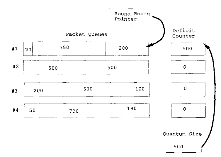
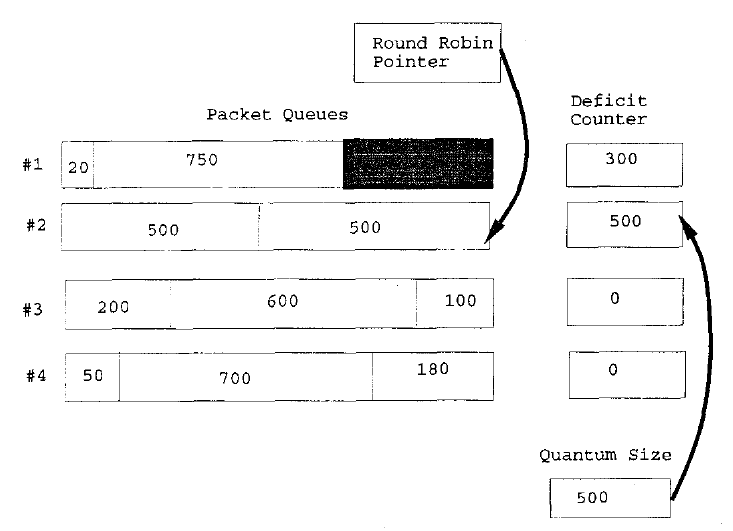
Figure 23. DRR queues with deficit counter from [Shreedhar1996].

Figure 24. DRR round pointer advancement from [Shreedhar1996].

Figure 24 shows the result when the round robin pointer goes to the next queue that needs servicing. We see that the first deficit counter has been decremented and that the second queue's deficit counter has been incremented by the "quantum size". This process continues and achieves long term fairness amongst all active flows regardless of the flows packet lengths. To offer differing long term bandwidth guarantees we can assign flow i a quantum size $Q_i$ to be used in each round then in the long term if there are N flows, flow i will receive a rate of

$$\frac{Q_i}{Q_1 + Q_2 + \ldots + Q_N}R$$

where $R$ is the line rate. As discussed in [Shreedhar1996] DRR does well in achieving fairness in bandwidth allocation amongst the flows and its computational efficiency allows for very fast hardware implementation. However DRR does not provide tight delay bounds since a packet from a flow that previously was not sending may get stuck waiting for an entire round where every other active flow gets its quantum and any that was remaining. It is in this case that WFQ and HFSC shine. However, on a high speed port even this worst case scenario may not result in significant delays depending on the number of queues and the port speed.

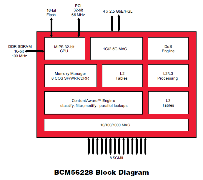
Like so many of the other queueing disciplines we've seen DRR is available in Linux, i.e., try man tc-drr. However, unlike the previous queueing disciplines this one shows up in switch chips as we see below in the memory manager portion of the block diagram of Figure 25. Like so many of the other queueing disciplines we've seen DRR is available in Linux, i.e., try man tc-drr. However, unlike the previous queueing disciplines this one shows up in switch chips as we see below in the memory manager portion of the block diagram of Figure 25.

Figure 25. Switch chip with DRR in the memory manager.

Priority Queueing

For an even simpler scheduling discipline that is readily implementable in high speed hardware and software too, we have priority queueing. Here we typically have 2, 4, or 8 levels of priority with each priority getting a queue. Packets from a lower priority queue do not get sent while there are packets in a higher priority queue. This provides a simple method of isolating flows and is typically used with along with packet header fields such as Ethernet's priority code point (PCP) or IP's differentiated services code points (DSCP) to simply place a packet into the appropriate queue rather than having to do a computationally costly classification phase. In the previous switch chip block diagram, Figure 25, this was the meaning of the "8 COS SP" in the memory manager, i.e., 8 classes of service or service priorities. And yes Linux does have a very general priority scheduler see man tc-prio.

Network Models for QoS

So far we've studied a number mechanisms for enhancing QoS in networks. In most cases so far we've only applied them in the context of a single link. The exception being the delay, jitter, and queue size bounds for the Virtual Clock and WFQ packet schedulers. Now we will take a look at two fundamentally different network QoS models: (a) the Integrated Services Internet, and (b) Differentiated Services.

Integrated Services Internet QoS Model

The Integrated Services Internet (IntServe) was standardized at the IETF by the now concluded IntServe working group. IntServe featured a general notion of flow like that we've seen in MPLS forwarding equivalence classes and SDNs. The key features of the IntServe architecture are:

Flow QoS Specification/Traffic Characterization

"In order to state its resource requirements, an application must specify the desired QoS using a list of parameters that is called a flowspec. The flowspec is carried by the reservation setup protocol, passed to admission control for to test for acceptability, and ultimately used to parametrize the packet scheduling mechanism."
Per Node Reservations
1. Reservation setup protocol
  
  This was where the RSVP protocol we saw in MPLS and GMPLS originated. RSVP would be used to carry the QoS reservation request from node to node along the path that would be taken by the packets.
2. Admission Control
  
  “Admission control implements the decision algorithm that a router or host uses to determine whether a new flow can be granted the requested QoS without impacting earlier guarantees. Admission control is invoked at each node to make a local accept/reject decision, at the time a host requests a real-time service along some path through the Internet.”
Per Node Behavior
1. Classifier
  
  “For the purpose of traffic control (and accounting), each incoming packet must be mapped into some class; all packets in the same class get the same treatment from the packet scheduler.”
2. Packet Scheduling
  
  “The packet scheduler manages the forwarding of different packet streams using a set of queues and perhaps other mechanisms like timers.”

Most of the authors of the IntServe documents were aware of the power of the packet scheduling algorithms such as Virtual Clock, WFQ, HFSC, in fact some of the authors invented them. Hence the emphasis on per node configuration of flow QoS guarantees via RSVP and the process of admission control to insure that the parameters for the packet scheduler could be properly set to acheive the desired QoS guarantees. IntServe did not put much emphasis on policing since, as we've seen, the sophisticated packet schedulers provide protection against badly behaving flows as well as delay bounds.

As to why IntServe didn't see wide adoption there are many reasons: (a) IntServe required "state" information to be kept at each router for each QoS flow traversing it, which could lead to scaling problems, (b) Sophisticated packet schedulers required significant computation capability so were not easily available at high speeds, (c) lack of a clear business model, recall this was before VoIP took off, and (d) a readily available (and more profitable for equipment vendors) alternative of "throwing bandwidth" at the problem. A list of key IntServe RFCs follows:

ID	Name	Date	Type
RFC1633	Integrated Services in the Internet Architecture: an Overview	6/1994	Informational
RFC2210	The Use of RSVP with IETF Integrated Services	9/1997	Standards Track
RFC2211	Specification of the Controlled-Load Network Element Service	9/1997	Standards Track
RFC2212	Specification of Guaranteed Quality of Service	9/1997	Standards Track

Differentiated Services Internet Model

If one can intuitively understand the Integrated Internet Services model as an elaborate infrastructure to take advantage of sophisticated packet schedulers, then one can understand the Differentiated Services (DiffServ) model as an elaborate infrastructure set up to take advantage of simple 4 or 8 level priority scheduling mechanisms (the very last packet scheduling mechanism we looked at). The DiffServ model was standardized by the IETF's, now concluded, DiffServ working group.

To motivate the DiffServ approach to supporting QoS let's design a scheme to give good QoS to four types of packet traffic: (i) VoIP (low rate, delay sensitive), (ii) video conferencing (moderate rate, delay sensitive), (iii) video streaming (moderate rate, delay insensitive, drop sensitive) and (iv) file transfer (high rate, delay insensitive, very drop sensitive). Given only a simple priority packet scheduler and queue limit control we could assign priorities and queue limits as follows:

Low rate, Delay Sensitive Traffice (VoIP) ⇒ Highest priorty, with small queue limit to prevent delays from getting large.
Moderate rate, Delay Sensitive Traffic (Video conf) ⇒ Second highest priority, with a small queue limit again
Moderate rate, Delay Insensitive Traffic, Drop sensitive ⇒ 3rd highest priority, with medium to large queue limits to avoid packet loss.
High but adjustable rate, Delay insensitve, Very Drop sensitive ⇒ 4th highest priority, with the largest queue limits.

The general principle here is to map delay sensitive traffic to queues with small buffer sizes, but since they have small buffers we need to give them high priority otherwise the delay sensitive traffic packets would build into a potentially long queue and get dropped if made to wait behind other traffic. Such a scheme can work well only if:

We know something about the traffic characteristics of the first three classes that want bandwidth guarantees. We've seen how to do this with our $(\sigma, \rho)$, burst and average rate characterization.
We can control the number of flows that are in each class that have hard bandwidth and delay requirements. We also know the total link bandwidth. This is the admission control process and our earlier bounds for flows through a multiplexer can be applied in making the admission decision.
We can make sure that traffic from a flow in a particular class is behaving in a reasonable way. For example if a flow claims to be VoIP traffic we should not see a packet rate of 50Mbps from this flow as such a rate is way out of line with the expected 100kbps expected. This is important since with our simple priority scheduler there is no protection from other flows within the same class. We saw how to do this via the policing mechanism (srTCM, trTCM) that we learned about earlier.

This is the essence of the Differentiated Services architecture. From RFC2475:

“This architecture achieves scalability by implementing complex classification and conditioning functions only at network boundary nodes, and by applying per-hop behaviors to aggregates of traffic which have been appropriately marked using the DS field in the IPv4 or IPv6 headers.”

“The differentiated services architecture is based on a simple model where traffic entering a network is classified and possibly conditioned at the boundaries of the network, and assigned to different behavior aggregates. Each behavior aggregate is identified by a single DS codepoint. Within the core of the network, packets are forwarded according to the per-hop behavior associated with the DS codepoint.”

Two general class of per hop behavior have been defined for the differentiated services architecture "Expedited Forwarding" and "Assured Fowarding". Expedited forwarding roughly seeks to offer average throughput (rate) guarantees while assured forward provides for a small number different service classes and packet treatment.

Expedited Forwarding PHB (RFC3246)

“The intent of the EF PHB is to provide a building block for low loss, low delay, and low jitter services. The details of exactly how to build such services are outside the scope of this specification.”
“To ensure that queues encountered by EF packets are usually short, it is necessary to ensure that the service rate of EF packets on a given output interface exceeds their arrival rate at that interface over long and short time intervals, independent of the load of other (non-EF) traffic. This specification defines a PHB in which EF packets are guaranteed to receive service at or above a configured rate and provides a means to quantify the accuracy with which this service rate is delivered over any time interval. It also provides a means to quantify the maximum delay and jitter that a packet may experience under bounded operating conditions.”

Assured Forwarding PHB (RFC2597)

“Assured Forwarding (AF) PHB group is a means for a provider DS domain to offer different levels of forwarding assurances for IP packets received from a customer DS domain. Four AF classes are defined, where each AF class is in each DS node allocated a certain amount of forwarding resources (buffer space and bandwidth). IP packets that wish to use the services provided by the AF PHB group are assigned by the customer or the provider DS domain into one or more of these AF classes according to the services that the customer has subscribed to.”
“Within each AF class IP packets are marked (again by the customer or the provider DS domain) with one of three possible drop precedence values. In case of congestion, the drop precedence of a packet determines the relative importance of the packet within the AF class. A congested DS node tries to protect packets with a lower drop precedence value from being lost by preferably discarding packets with a higher drop precedence value.”
“In a DS node, the level of forwarding assurance of an IP packet thus depends on (1) how much forwarding resources has been allocated to the AF class that the packet belongs to, (2) what is the current load of the AF class, and, in case of congestion within the class, (3) what is the drop precedence of the packet.”
“Assured Forwarding (AF) PHB group provides forwarding of IP packets in N independent AF classes. Within each AF class, an IP packet is assigned one of M different levels of drop precedence. An IP packet that belongs to an AF class i and has drop precedence j is marked with the AF codepoint AFij, where 1 <= i <= N and 1 <= j <= M. Currently, four classes (N=4) with three levels of drop precedence in each class (M=3) are defined for general use. More AF classes or levels of drop precedence MAY be defined for local use.”

ID	Name	Date	Type
RFC2475	An Architecture for Differentiated Services	12/1998	Informational
RFC2474	Definition of the Differentiated ServicesField (DS Field) in theIPv4 and IPv6 Headers	12/1998	Standards Track
RFC3246	An Expedited Forwarding PHB (Per-Hop Behavior)	3/2002	Standards Track
RFC2597	Assured Forwarding PHB Group	6/1999	Standards Track

References

[Arfeen2013] M. A. Arfeen, K. Pawlikowski, D. McNickle, en A. Willig, “The Role of the Weibull Distribution in Internet Traffic Modeling”, in Teletraffic Congress (ITC), 2013 25th International, 2013, bll 1–8
[Cruz1991] R. L. Cruz, “A Calculus for Network Delay. I. Network Elements in Isolation”, Information Theory, IEEE Transactions on, vol 37, no 1, bll 114–131, 1991.
[Bertsekas1992] D. P. Bertsekas, Network Optimization: Continuous and Discrete Models. Athena Scientific, 1998.
[HZhang1995] H. Zhang, “Service Disciplines for Guaranteed Performance Service in Packet-Switching Networks”, Proceedings of the IEEE, vol 83, no 10, bll 1374–1396, 1995.
[McKenney1990] P. E. McKenney, “Stochastic Fairness Queueing”, in INFOCOM’90, Ninth Annual Joint Conference of the IEEE Computer and Communication Societies. The Multiple Facets of Integration. Proceedings, IEEE, 1990, bll 733–740.
[Shreedhar1996] M. Shreedhar en G. Varghese, “Efficient Fair Queueing Using Deficit Round Robin”, SIGCOMM Comput. Commun. Rev., vol 25, no 4, bll 231–242, 1995.
[LZhang1990] L. Zhang, “Virtual Clock: A New Traffic Control Algorithm for Packet Switching Networks”, in ACM SIGCOMM Computer Communication Review, 1990, vol 20, bll 19–29.
[Parekh1993] A. K. Parekh en R. G. Gallager, “A Generalized Processor Sharing Approach to Flow Control in Integrated Services Networks: The Single-Node Case”, IEEE/ACM Transactions on Networking, vol 1, no 3, bll 344–357, Jun 1993.
[Stoica2000] I. Stoica, H. Zhang, en T. S. E. Ng, “A Hierarchical Fair Service Curve Algorithm for Link-Sharing, Real-Time, and Priority Services”, IEEE/ACM Transactions on Networking, vol 8, no 2, bll 185–199, Apr 2000.