MPLS Origins

If we included non-electronic forms of networking, e.g., mail or package handling networks then we reached the conclusion that connectionless packet switching where each packet contains the full destination address of the recepient was far older than circuit switching. However, in the electronic era analog voice circuit switching preceeded any form of electronic message switching by many decades. However it wasn't long after the first digital voice circuits and hierarchies were deployed that the very first commercial digital packet switching systems were developed. Such systems were developed under extreme hardware processing constraints.

Minimum Multiplexing of Packets

In going from a TDM or FDM (frequency division multiplexing) system to one based on packet multiplexing — sometimes refered to as statistical multiplexing — we need some way to tell apart packets bound for different destinations on a link. In IP and Ethernet we just use addresses, however these were far too long to be processed by early digital hardware. At a minimum we need to label a packet so that we can enable multiplexing and demultiplexing, i.e., we can tell one packet apart from other packets bound for different destinations on the same link. This led to a connection oriented form of packet switching based on labels with the following properties.

• Labels only need to be unique on a per link basis and not a per network basis.
• Labels could be reused after a connection using that label was torn down. This was in analogy with circuit switching where phone connections would reuse trunk timeslots as connections were torn down and setup.
• Based on the above labels could be much shorter than the number of possible destination addresses since addresses need to be network wide unique and cannot be reused.

Historical Examples:

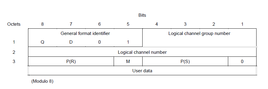
• In X.25, Figure 1, there were two levels of labels. The logical channel number — 8 bits — and the logical channel group number — 4 bits.
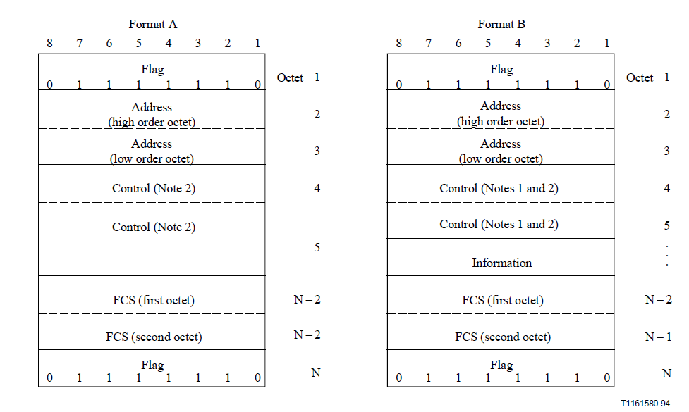
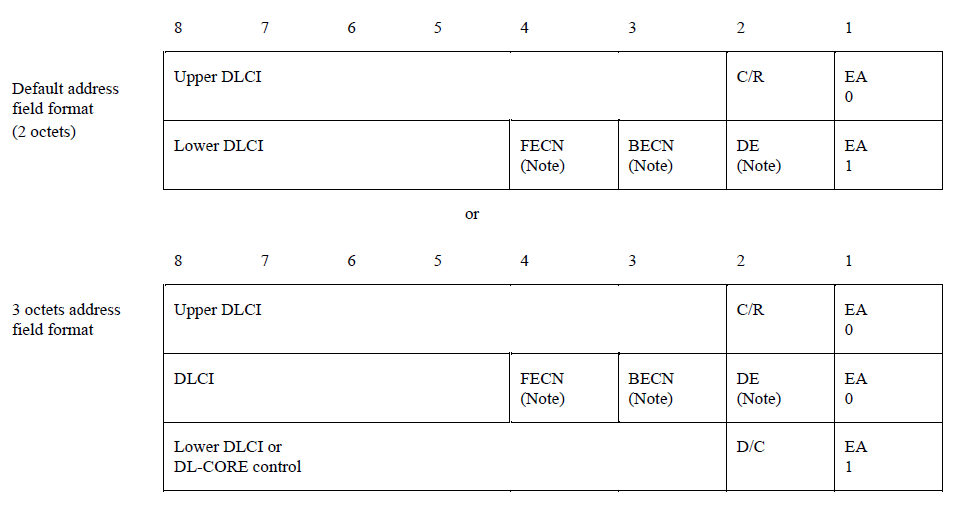
• In Frame Relay, Figures 2 and 3, the label is called the Data Link Connection Identifier and could be either 10, 16, 19, or 25 bits long.
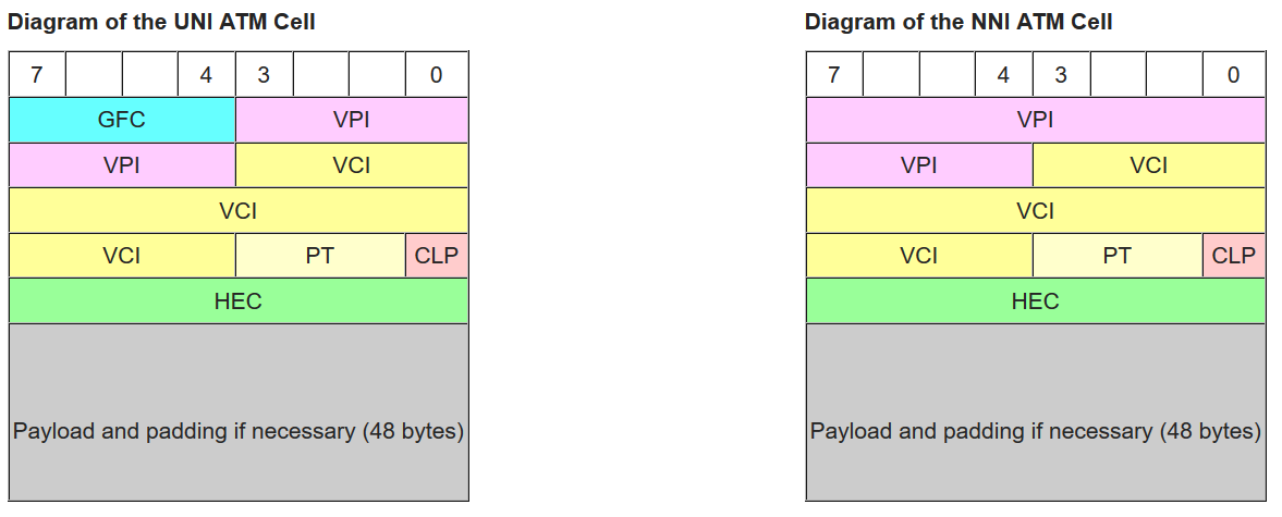
• In ATM, Figure 4, there are two levels of labels known as the Virtual Path Identifier (VPI) — 12 bits — and the Virtual Channel Identifier (VCI) — 16 bits.

In the above list and figures you may have noticed that in Frame Relay and ATM the size of the "labels" were starting to get rather large. Doesn't this counter the idea of small labels for fast hardware processing? Actually not. Unlike an IP router or an Ethernet switch that must be able to forward a packet as long as it has a "legal" address. Switches that work with labels are allowed to support only a limited range of labels. Hence the specifications show the maximum number of labels that ever could be supported.

To enable data to flow from source to destination in a label switched — connection oriented — packet network we need to set up a connection, i.e., set up appropriate forwarding tables on each switch along the path. In the process of doing this we must pay attention to label restrictions on each switch along the path. We'll see this idea again in GMPLS for optical networks where the "labels" are extremely constrained.

Aside: Over the years the general notion of label switching has used a number of other names including : Virtual Circuits, Connection Oriented Packet Switching, and Tag switching.

Label Switched Networking

Consider the network shown in Figure 5 consisting of five switches and ten hosts. We'll use this network to illustrate the basics of label switched networking.

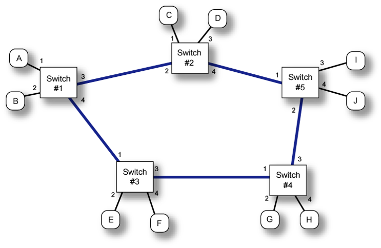
Suppose that the following hosts wish to communicate with each other: Host A to Host J, Host B to Host C, Host E to Host I, Host D to Host H, and Host A to Host G. The first thing we would need to do is select paths across the network for each communicating pair. One has a great deal of flexibility in the choice of path as we'll discuss later. For now consider the paths shown in the Figure 6.

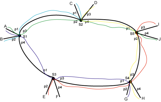
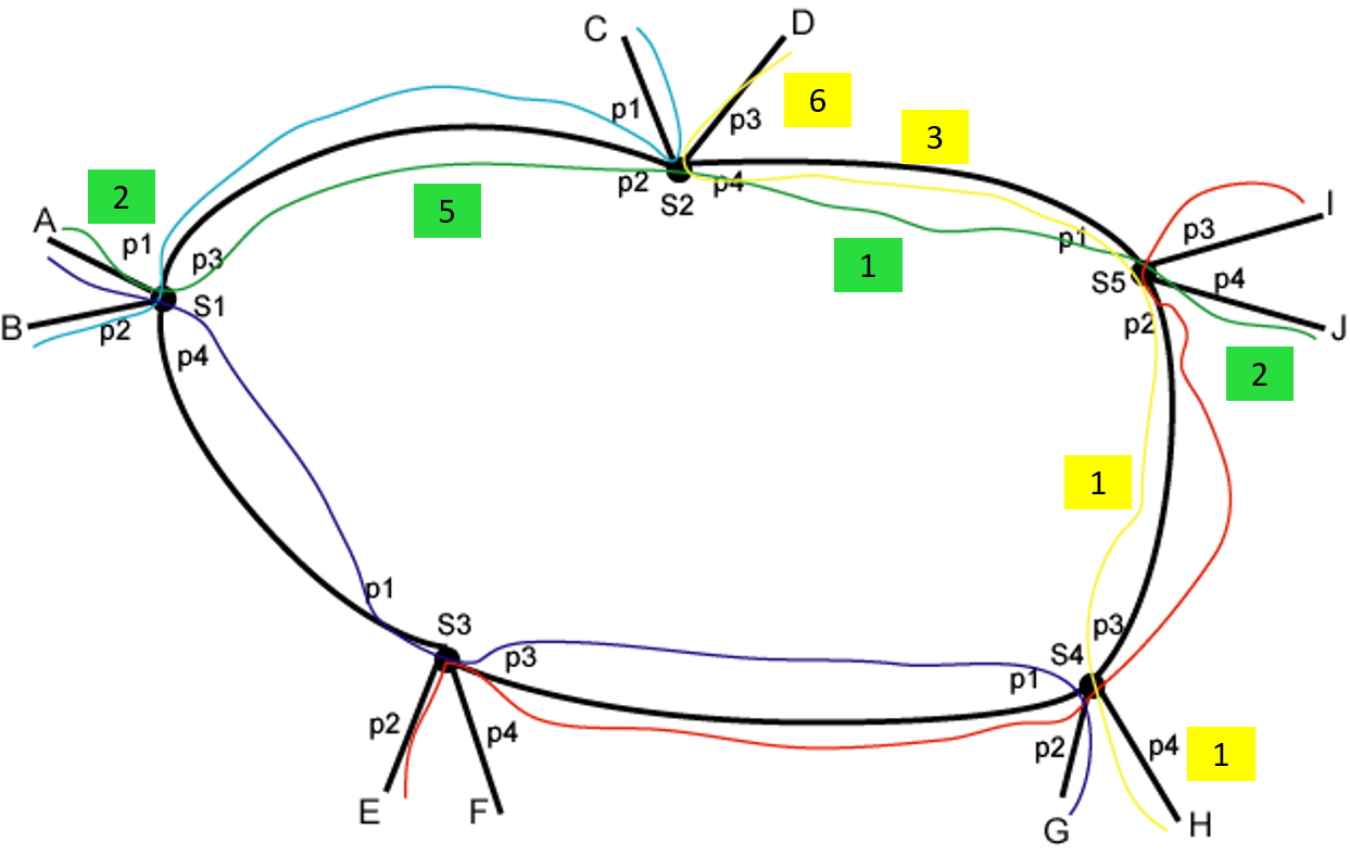
The next step is to choose a label for each segment of a label switched path (LSP). By this we mean for each link that a particular LSP traverses we need a label so that we can tell packets from this LSP apart from other LSPs that may be using the same link. Recall: Labels only need to be unique on a link. They are not an address and have no network-wide or switch-wide significance. In Figure 7 we show (somewhat arbitrary) label assignments for the LSPs between hosts A-J and D-H:

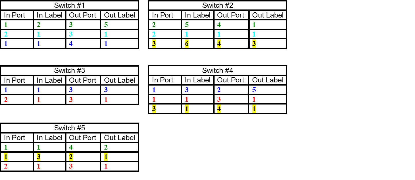
With the labels assigned we can now set up the label switching forwarding tables on each switch, Figure 8. These consists of a map of tuples (in port, in label) to (out port, out label). We frequently call an individual element of a label switch forwarding table a cross-connect (xconnect).

Question: In the worst case how many bidirectional virtual circuits do we need in a network with N endpoints? Answer: $$Count_{LSP} = \frac{N(N-1)}{2}$$

Question: How many entries are there in a switches forwarding table? Answer: There is an entry in the forwarding table for each LSP that traverses that particular switch and NOT for each LSP in the network.

Datagram and Label Switching Compared

In datagram switching — also known as connecitonless packet switching — switching is based on addresses. In this class we use Ethernet and IP as examples of datagram switching. In the most commonly implemented form of datagram switching, switching is based on destination address only. As a reminder network addresses are generally network-wide unique. In Figure 9 we show a set of possible datagram forwarding tables.

Question: How many entries does the forwarding table of a datagram switch (aka IP router) theoretically need? Answer: One for every endpoint (destination) in the network, i.e., N entries.

Question: In practice how does one reduce the number of entries in an IP routing table? Answer: Default routes and address summarization/aggregation.

Recomended Readings

From the MPLS Architecture document, RFC3031 see the following sections:

• 2.1 Overview (required reading),
• 3.1 Labels,
• 3.3 Labeled Packet,
• 3.4 Label Assignment and Distribution,
• 3.6 Label Distribution Protocols (in general),
• 3.9 The Label Stack,
• 3.10 NHLFE,
• 3.11 Incoming Label Map,
• 3.12 FEC-to-NHLFE Map,
• 3.13 Label Swapping,
• 3.14 Scope and Uniqueness of Labels (a bit difficult to read),
• 3.15 Label Switched Path (LSP),
• 3.21 Route Selection,
• 3.27 Tunnels and Hierarchy (in particular Hierarchy: LSP Tunnels within LSPs)

MPLS Data Plane

The MPLS Label

The MPLS label stack entry is defined in RFC3032:

 0                   1                   2                   3
 0 1 2 3 4 5 6 7 8 9 0 1 2 3 4 5 6 7 8 9 0 1 2 3 4 5 6 7 8 9 0 1
+-+-+-+-+-+-+-+-+-+-+-+-+-+-+-+-+-+-+-+-+-+-+-+-+-+-+-+-+-+-+-+-+ Label
|                Label                  | Exp |S|       TTL     | Stack
+-+-+-+-+-+-+-+-+-+-+-+-+-+-+-+-+-+-+-+-+-+-+-+-+-+-+-+-+-+-+-+-+ Entry

                    Label:  Label Value, 20 bits
                    Exp:    Experimental Use, 3 bits
                    S:      Bottom of Stack, 1 bit
                    TTL:    Time to Live, 8 bits

                              Figure 1

We see that the label is quite long, 20 bits, giving us the potential for lots of LSPs on any particular link. Similar to IP the label stack entry contains a time to live (TTL) field to guard against loops. As one might guess from the name that the label stack entries can be "stacked" to produce nested LSPs (multiplex hierarchies) which we'll study in a bit.

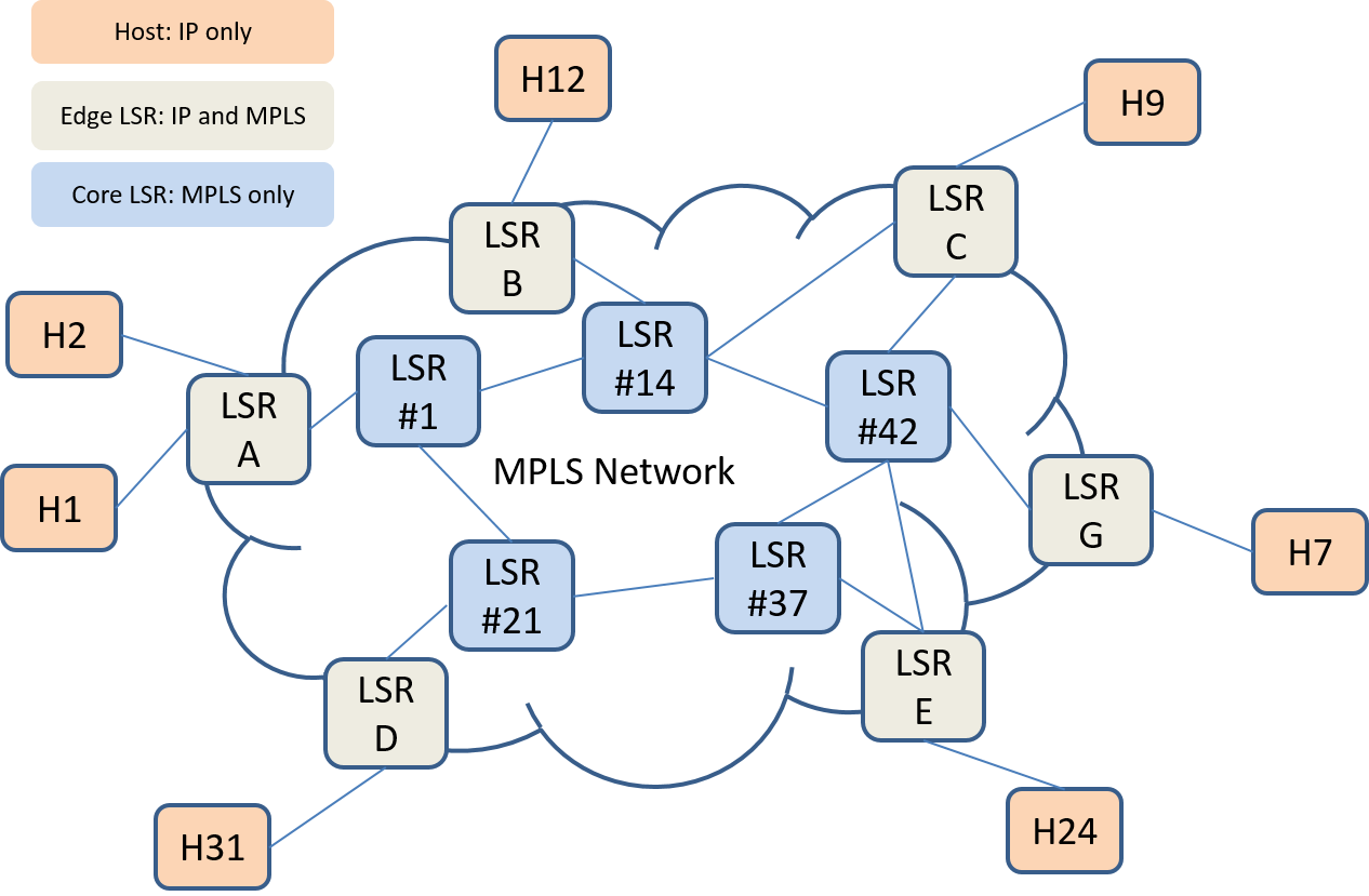
MPLS Network elements LSRs at the core and edge

Unlike past label switching (virtual circuit) technologies MPLS was specifically architected to work with IP. In particular Edge Label Switched Routers (E-LSRs) are required to be able to work with IP only hosts and subnetworks while the LSRs in the core of an MPLS network only need to switch based on labels. This is illustrated in Figure 10.

Getting IP packets into and out of LSPs

On ingress (enterance) to an MPLS network the E-LSR (edge LSR) pushes labels onto the front of an IP packet so that the core LSRs only need to switch based on that label. On egress (exit) from the MPLS network the E-LSR pops (removes) the label from the front of the IP packet before forwarding the packet on to an IP host or subnetwork.

We call the group of IP packet streams (or flows) that are forwarded in the same manner a forwarding equivalence class (FEC). Do not confuse this with "forward error correction (FEC)" these are completely different things working at very different layers. It is the job of the ingress LSR (on the boundary of the MPLS network) when receiving an IP packet to “classify” it into an FEC, then, “push” the label of the corresponding FEC onto that IP packet for transport on the MPLS network.

How can one classify IP packets into FECs? RFC3814 (MPLS management) lists the following packet header information that can be used in classification:

1. IP source address range  → Breaks IP destination based forwarding paradigm

2. IP destination address range

3. Source port range (UDP, TCP, etc.)  →  Layer 4 information

4. Destination port range (UDP, TCP, etc.) → Layer 4 information

5. IPv4 protocol field (IPv6 next header field) → Layer 4 information

6. DiffServ Code Point (DSCP) → QoS related information. We’ll learn about this towards the end of the course.

Could one look at more fields in the incoming packet? Yes. What would marketing have to say about that? We’ve invented Layer 4, Layer 6, Layer 7 switching! We'll also see an extension of these classification fields when we look at the OpenFlow protocol for Software Defined Networks (SDNs).

LSP Merging

Previously we saw a need for approximately N^2^ LSPs for full communications between N endpoints. As there are techniques to reduce IP forwarding table size, there are techniques to reduce the number of LSP cross connects in an LSR. The simplest of these is the concept of LSP merging. Consider the network shown in Figure 11 with three LSPs highlighted.

In this figure we see LSPs defined between LSRs A-C, D-C, and E-C. Per our previous rules we could use the following label assignments:

• LSP A-C: (Link A-1, Label 1), (Link 1-14, Label 17), (Link 14-42, Label 10), (Link 42-C, Label 3)
• LSP D-C: (Link D-21, Label 1), (Link 21-1, Label 2), (Link 1-14, Label 18), (Link 14-42, Label 11), (Link 42-C, Label 4)
• LSP E-C: (Link E-37, Label 4), (Link 37-14, Label 1), (Link 14-42, Label 12), (Link 42-C, Label 5)

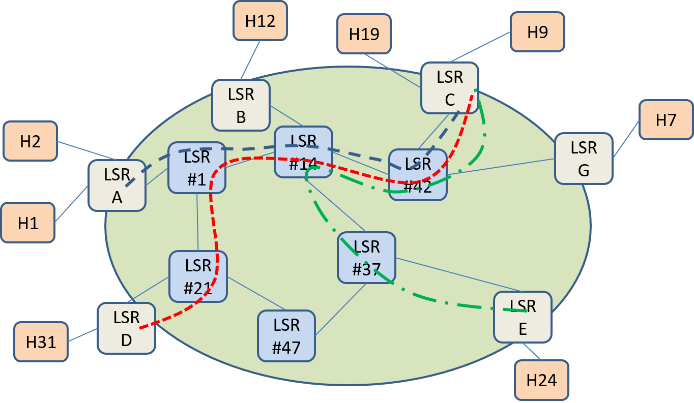
Can we be more efficient? If MPLS is carrying IP packets, as is the case here, we note that all these LSPs terminate at LSR C where the label is popped and the IP packets are forwarded on to hosts or subnets. Hence we still have IP addresses as "demultiplexing" information to help us tell them apart at E-LSR C. It seems that we don't need to keep three distinct LSPs throughout the network but could merge LSPs at LSR #1, LSR #14, LSR #42 as shown in Figure 12.

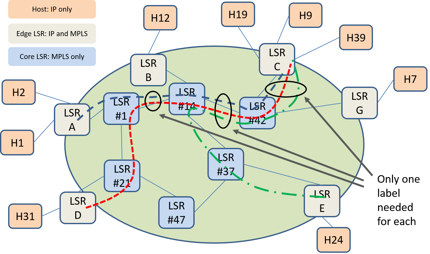
We can now use a simplified label assignment that results in smaller LSP tables on the switches (overlapping label assignments in italics):

• LSP A-C: (Link A-1, Label 1), (Link 1-14, Label 17), (Link 14-42, Label 10), (Link 42-C, Label 3)
• LSP D-C: (Link D-21, Label 1), (Link 21-1, Label 2), (Link 1-14, Label 17), (Link 14-42, Label 10), (Link 42-C, Label 3)
• LSP E-C: (Link E-37, Label 4), (Link 37-14, Label 1), (Link 14-42, Label 10), (Link 42-C, Label 3)

Multiplexing hierarchies via Label Stacks

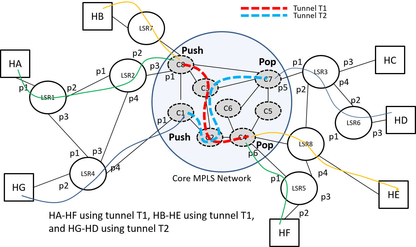
The ability to merge LSPs requried that the LSPs had a common destination. If the LSPs just have a section of overlap we can apply a different technique that of label stacking — LSP nesting — to save on LSR table entries. Consider Figure 13 below with LSPs defined between HA-HF and HB-HE. This figure also illustrates a common division of a network into a core and edge subnetworks. Some observations:

• Core network LSRs suffer most from the N^2^ LSP connectivity problem since they provide connectivity to potentially many more endpoints than an edge network.
• Core network LSRs generally need to be faster (higher capacity) than edge network LSRs.
• There is a limited number of "good" paths across any network especially the core network. For example the paths produced by a k-shortest path algorithm or diverse path algorithm.

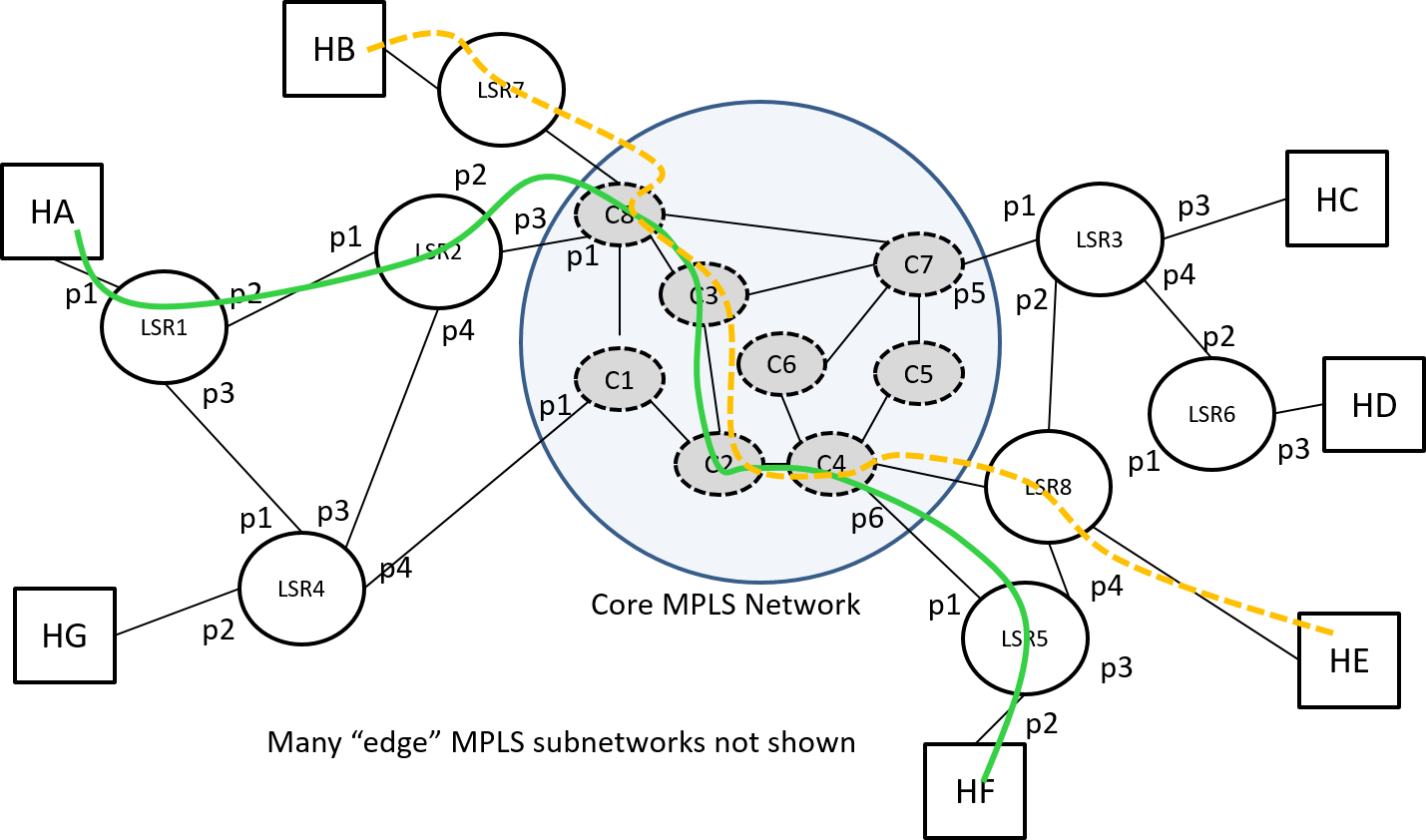
To reduce the number of LSPs needed in the core network we can set up tunnels for various popular paths across the core network and then put the end-to-end LSPs through the appropriate core tunnels. This is done by utilizing a stack of labels rather than just a single label. In Figure 14 we show part of the overlap of the previous LSPs replace by a tunnel across the core and indicate where additional label push and pop operations occur within the core network.

Summary of MPLS Data Plane Operations

Fundamental Label Switching Operations:

1. Classification – Initial label push on entering the MPLS network

2. Label Push – When "multiplexing" an LSP into a tunnel (may be repeated)

3. Label Pop – When demultiplexing an LSP from a tunnel (may be repeated)

4. Egress Label Pop – When removing the last label on exiting the MPLS network

5. Label Swap – When switching MPLS packets at MPLS nodes

From the above list we see that the "instructions" that the forwarding plane gets from its "forwarding table" is more complicated than an (input port, input label) to (output port, ouput label) mapping. In the MPLS archtecture RFC3031 they call this "forwarding instruction" a Next Hop Label Forwarding Entry (NHLFE).

Link Layers

MPLS does not have a specific specific link layer/physical layer! In fact MPLS's control plane was first applied to Frame Relay and ATM networks utilizing those network's inherent labels. Since then MPLS' label stack has been specified for use with a number of standard link layer technologies:

1. PPP (https://www.iana.org/assignments/ppp-numbers/ppp-numbers.xhtml)

2. Data Link Layer Protocol value 0x0281 MPLS Unicast

3. MPLS Control protocol 0x8281

4. Ethernet (https://www.iana.org/assignments/ieee-802-numbers/ieee-802-numbers.xhtml)

5. EtherType MPLS 0x8847

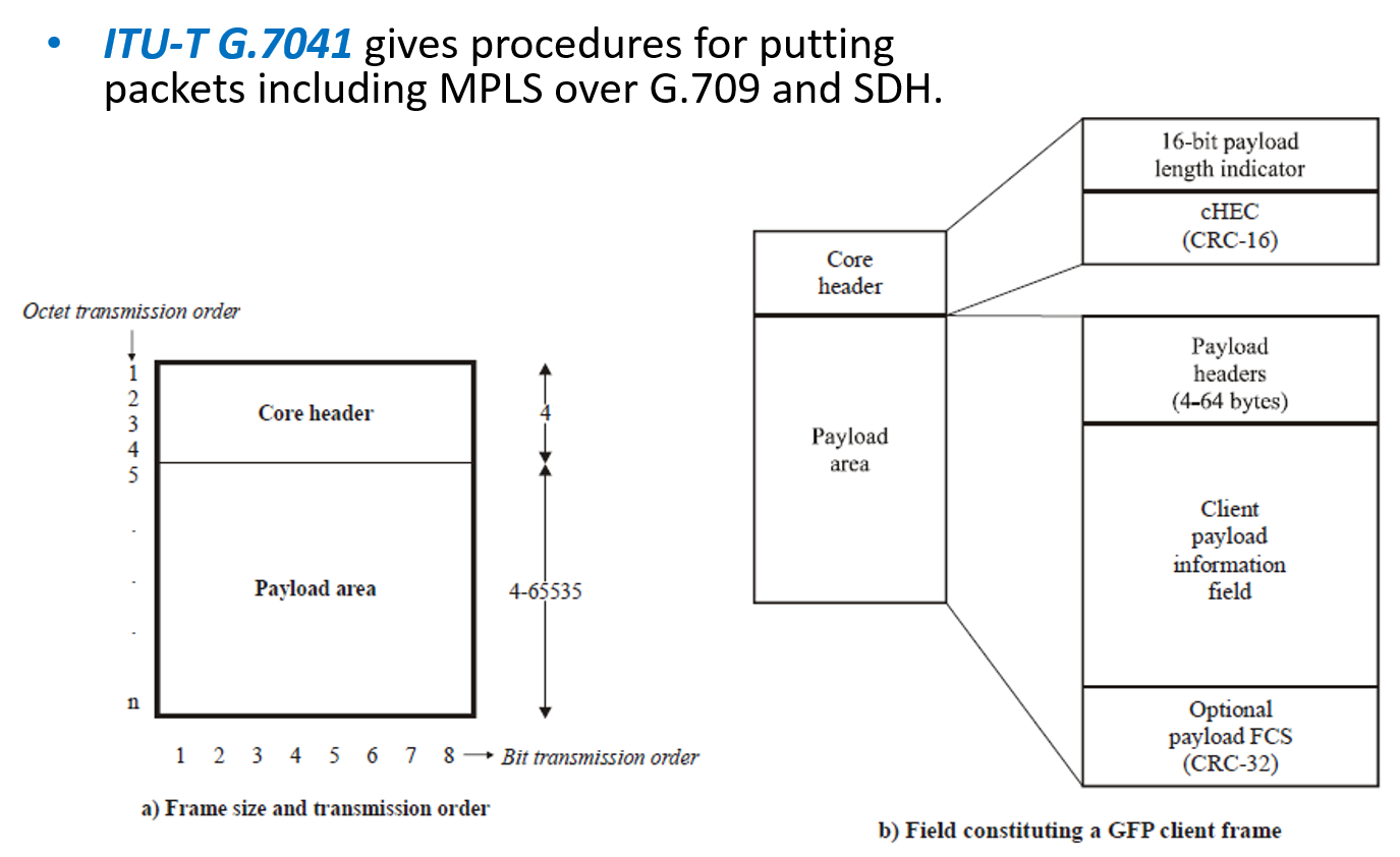
6. SDH/G.709 via GFP (G.7041)

7. Generic Framing Procedure type bits: 0000 1101

RFCs:

• RFC 2702 Requirements for Traffic Engineering Over, 1999-09.
• RFC 3031 Multiprotocol Label Switching Architecture, 2001-01.
• RFC 3032 MPLS Label Stack Encoding, 2001-01.
• RFC 3034 Use of Label Switching on Frame Relay Networks Specification, 2001-01.
• RFC 3035 MPLS using LDP and ATM VC Switching, 2001-01.
• RFC 5036 LDP Specification, 2007-10.
• RFC 3037 LDP Applicability, 2001-01.
• RFC 3209 RSVP-TE: Extensions to RSVP for LSP Tunnels, 2001-12.
• RFC 3210 Applicability Statement for Extensions to RSVP for LSP-Tunnels, 2001-12.
• RFC 3469 Framework for Multi-Protocol Label Switching (MPLS)-based Recovery, 2003-02.

MPLS Network Capabilities

Traffic Isolation

How can I launch a DOS/DDOS attack against a host or subnetwork in an MPLS network? To do so would require creating multiple LSPs to that host or subnetwork. But since these are setup either via management or signaling (control plane) they would be refused. Hence MPLS networks are more resilient to many types of attacks. Another way to think about this is that MPLS provides increased isolation compared to datagram networks which makes it popular for the creation of VPNs.

Traffic Engineering

How could I make better use of network resources in an MPLS network versus an IP network? In many IP routing protocols one makes use of shortest path algorithms to compute and configure forwarding tables. In Figure 16 we show a network — loosely based on an actual network topology in China — where we have colored links on the shortest path tree to node n30 in red and links not on the shortest path tree are shown in green.

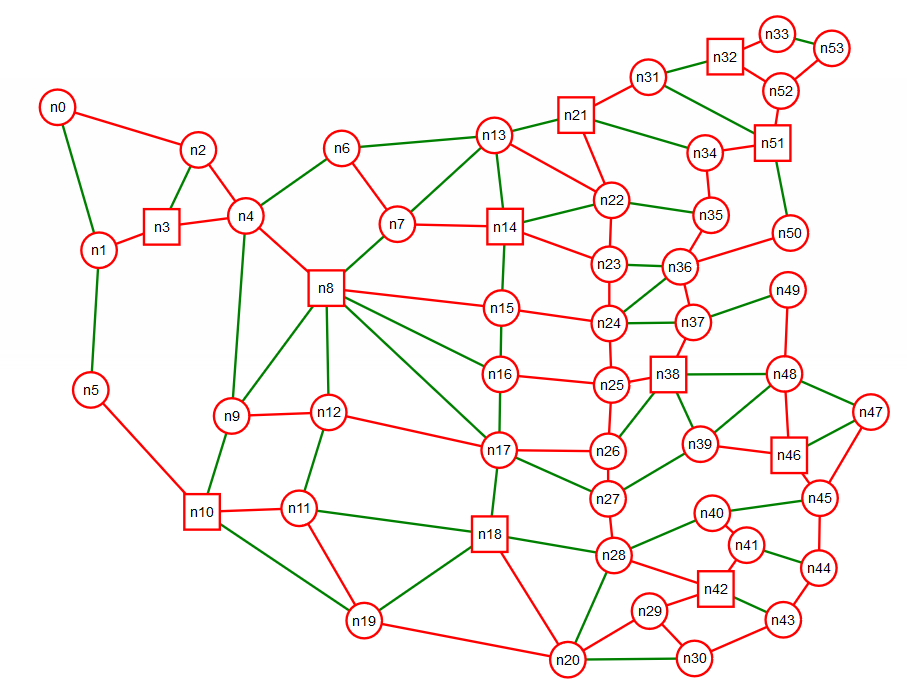
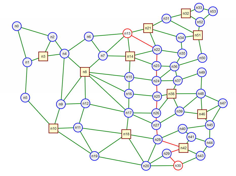
One thing we notice in this network is that many of the tree "branches" converge into a common trunk. This could lead to significant congestion on these "trunk" links. However it seems that there are a fair number of links not being used and that the cost in terms of distance for using those links might not be much worse that the shortest path. In Figure 17 we highlight just the links on the shortest path between nodes n13 and n30. The length of this shortest path in graphical units is 334.0.

Using a k-shortest path algorithm we can compute the 10 shortest paths, Figure 18, and see that the longest has a length of 368.7 units. Just slightly more than a 10% increase in length over the shortest path. Each of these additional 9 shortest paths avoids one or more links used by the shortest paths hence could possibly avoid a congested link.

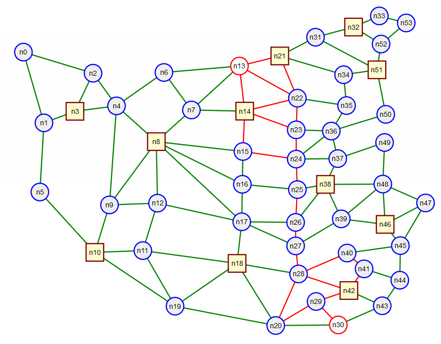
The process of choosing paths based on traffic conditions or demands is known as traffic engineering. MPLS's data plane being based on LSPs is well suited to traffic engineering, however, as we will see, not all MPLS control planes support traffic engineering. This is in contrast with destination based IP routing in which all paths to a destination must be part of a tree rooted on that destination.

MPLS Control Planes

The key ingredients to an MPLS control plane are:

1. “Routing” – (we cover Link State based routing here, e.g., OSPF, IS-IS)

   1. LSR/Router discovery – Hello protocol

   2. LSR/Router and link information sharing – Link state flooding

2. Path Computation

   1. The same as that used by IP in the LDP case, or
   2. Separate from the routing protocol for explicitly routed paths for traffic engineering and other purposes when using RSVP-TE signaling protocol.

3. Label Distribution

   1. LDP – Uses paths computed by route protocol, or

   2. RSVP-TE – for explicitly routed paths

Path Selection via the OSPF Routing Protocol

See slides for more figures and animations.

At a very high level, for a single area, and for point-to-point links only we can summarize the operation of a link state routing protocol such as OSPFv2 as follows:

• Nodes discover neighbors and the links connecting them to their neighbors
• Nodes advertise to their peers the links they know about (so every node has this information)
• Nodes can add additional information about links in their advertisements to peers.

These processes are done very efficiently and carefully:

• Nodes carefully “flood” information to peers
  • A node tags discovered link information with its “name” so that that peers know it came from you.
• Nodes don’t resend information back on the same interface it was received or to the same node that send it
  • Helps save network bandwidth (prevents infinite loops)
• Nodes don’t resend information that they receive that is tagged from themselves.
  • Further prevents infinite loops of information
• Nodes don’t resend duplicate information they receive
• Notes have a smart process to quickly bring a new neighbor node "up to speed", i.e., synchronization.

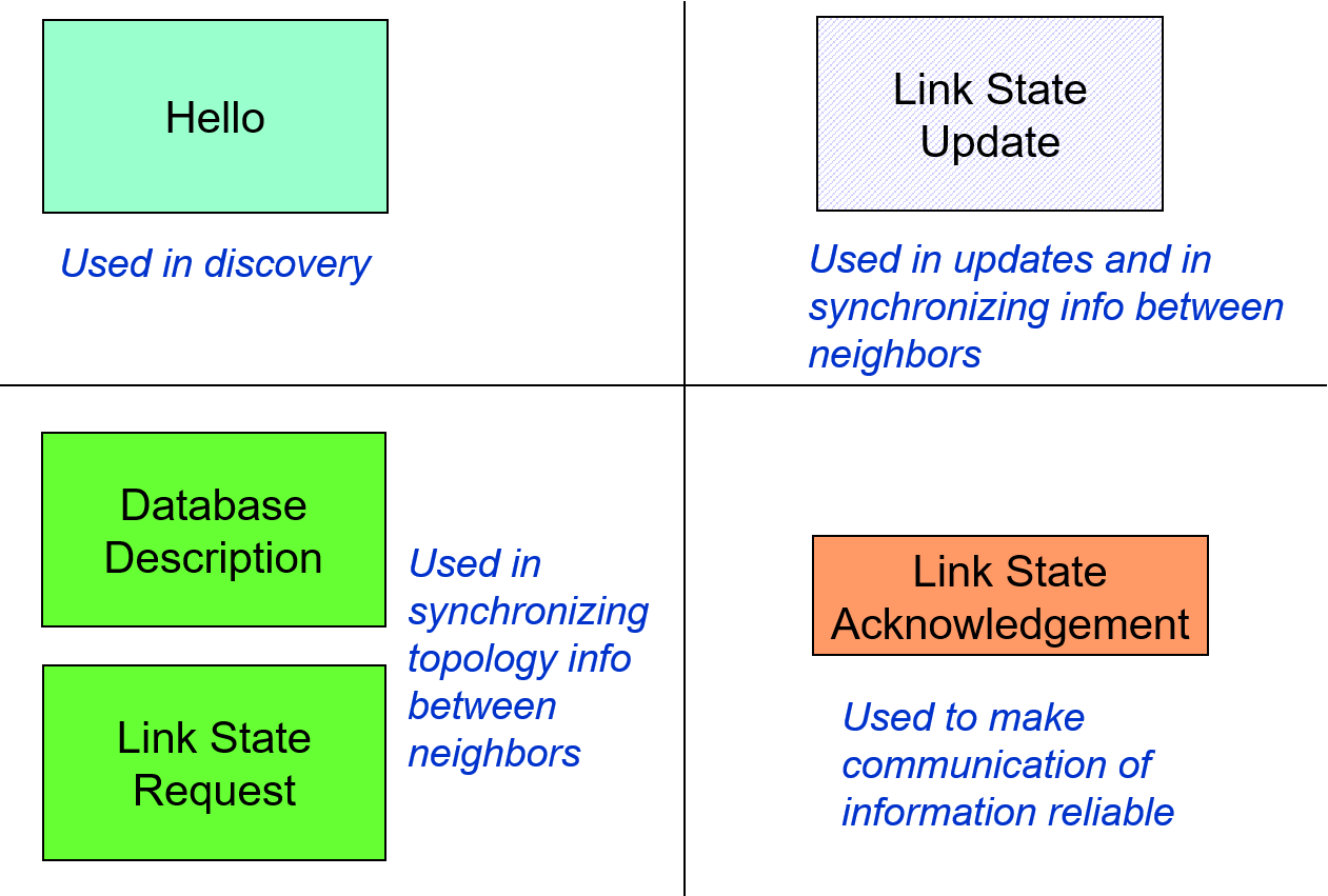
OSPF runs directly over IP and using the following packets:

The Label Distribution Protocol (LDP)

As we just saw we can use a routing protocol to discover LSRs and their connectivity, and if desired compute paths for potential LSPs. However we don't yet have a way to assign labels and fill in an LSR's forwarding table. This requires extra functionality that of "label distribution". There are currently three widely deployed approaches to label distribution: (a) The Label Distribution Protocol (LDP), (b) RSVP-TE (reservation protocol with traffic engineering extensions), (c) piggy backing label distribution on BGP (the border gateway routing protocol). We'll cover (a) and (b) in this course.

From Wikipedia:

“The Label Distribution Protocol (LDP) is a protocol defined by the IETF (RFC 5036) for the purpose of distributing labels in an MPLS environment. LDP relies on the underlying routing information provided by an IGP in order to forward label packets. The router forwarding information base, or FIB, is responsible for determining the hop-by-hop path through the network. Unlike traffic engineered paths, which use constraints and explicit routes to establish end-to-end Label Switched Paths (LSPs), LDP is used only for signaling best-effort LSPs.”

From the LDP standard RFC5036:

1. "LDP is a protocol defined for distributing labels. It is the set of procedures and messages by which Label Switched Routers (LSRs) establish Label Switched Paths (LSPs) through a network by mapping network-layer routing information directly to data-link layer switched paths."

2. 'LDP associates a Forwarding Equivalence Class (FEC) [RFC3031] with each LSP it creates. The FEC associated with an LSP specifies which packets are "mapped" to that LSP.'

3. 'LSPs are extended through a network as each LSR "splices" incoming labels for a FEC to the outgoing label assigned to the next hop for the given FEC.'

To accomplish its label distribution goals, LDP needs a fair amount of support functionality:

1. “LDP discovery is a mechanism that enables an LSR to discover potential LDP peers.” This is control plane discovery and is separate from the data plane discovery performed by OSPF or other IGP.

2. “LDP sessions exist between LSRs to support label exchange between them.”

3. “LDP uses TCP as a reliable transport for sessions.”

4. "There are four categories of LDP messages:"

   1. "Discovery messages, used to announce and maintain the presence of an LSR in a network."

   2. "Session messages, used to establish, maintain, and terminate sessions between LDP peers."

   3. "Advertisement messages, used to create, change, and delete label mappings for FECs."

   4. "Notification messages, used to provide advisory information and to signal error information."

How labels get assigned and distributed

Suppose we want to setup the LSP shown in Figure 20.

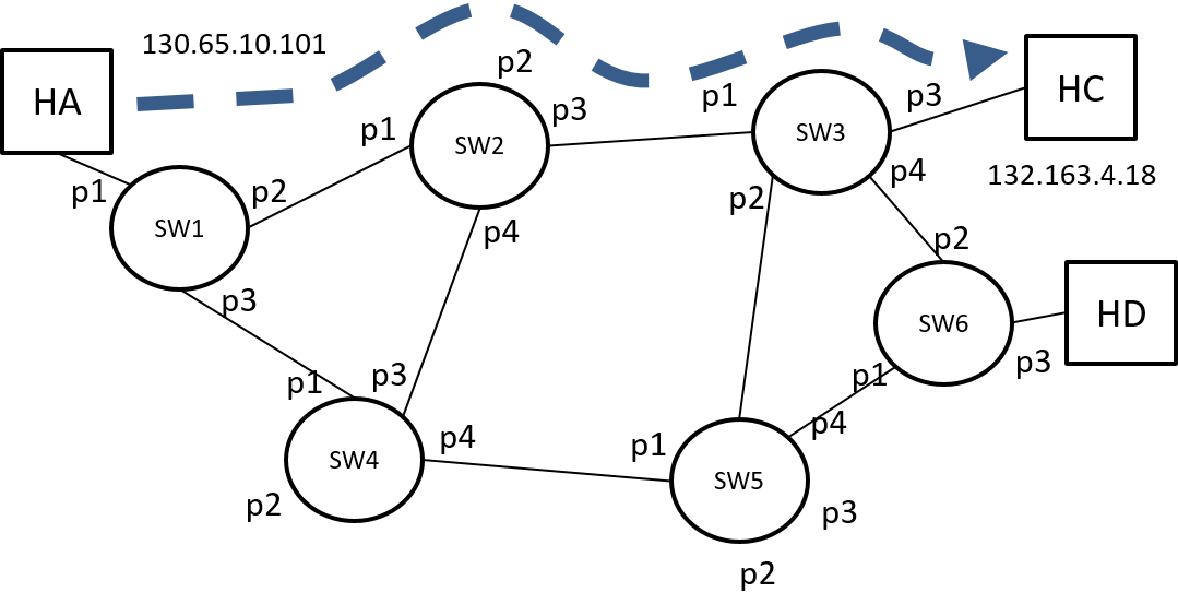
Here are a few things we need to keep in mind:

1. MPLS thinks in terms of unidirectional LSPs, i.e., a bidirectional connection would be thought of as two unidirectional LSPs.

2. Downstream is the direction of packet flow. Don't confuse this with the flow of "signaling" messages used to create the LSP.

3. Who should determine the label used on a link for a particular LSP?

4. Who has the harder “hardware” job the upstream or downstream LSR? Why? The upstream just needs to place a number in the header, while the downstream has to perform a look up based on the label, hence the downstream’s “hardware” job is harder so  it gets to choose the label.

5. Who knows about the FEC initially? The upstream LSR. Hence upstream LSR asks downstream LSR for a label.

6. From RFC3031: “Thus labels are downstream-assigned, and label bindings are distributed in the downstream to upstream direction.”

7. How does the upstream LSR know which downstream LSR to ask for a label?

8. It looks at its IP routing table. LDP uses the IP route tables to determine the LSPs path for the FEC.

9. This is good for setting up MPLS based IP VPNs to give customers isolation, but not useful for network traffic engineering.

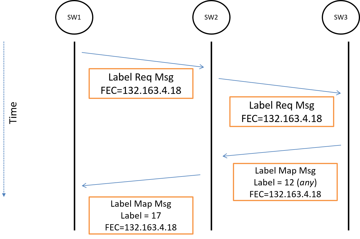
10. Simplified LDP Procedures:

11. “An LSR sends the Label Request message to an LDP peer to request a binding (mapping) for a FEC.”

12. “An LSR sends a Label Mapping message to an LDP peer to advertise FEC-label bindings to the peer.”

13. Ordered Label Distribution Control: “When using LSP Ordered Control, an LSR may initiate the transmission of a label mapping only for a FEC for which it has a label mapping for the FEC next hop, or for which the LSR is the egress.  For each FEC for which the LSR is not the egress and no mapping exists, the LSR MUST wait until a label from a downstream LSR is received before  mapping the FEC and passing corresponding labels to upstream LSRs.”

To illustrate the setup of an LSP in a network we can use a message sequence chart as shown in Figure 21.

RFC5037 (Experience with LDP Protocol):

“Nine of the 11 responses list Layer 3 Virtual Private Networks (L3VPNs) as the application driving the LDP deployment in the network.”

OSPF-TE

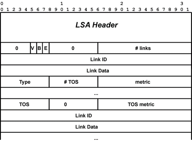
We saw in the overview of OSPF that there are Link State Update packets for communicating information about links in the network. Within those packets are "objects" called Link State Advertisements (LSAs) that carry information concerning particular types of links. Originaly OSPF defined the following LSAs:

• Router (LSA type 1)
• Network (LSA type 2)
• Summary (LSA type 3)
• ASBR (LSA type 4)
• External (LSA type 5)

For point to point links in a single OSPF area only the Router LSA is relevant to us now. Its format is shown in the figure below. In this figure we see that along with the data associated with a link is a "metric" field. (Note that multiple TOS fields were never widely used or deployed). This is the "weight" or "distance" number used in the shortest path computations.

One thing that we don't see in the Router LSA is any information to help with traffic engineering. What kind of information might be helpful?

• Bandwidth capability of the link
• Current bandwidth usage on a link
• Information on link reliability
• Etc...

To accommodate the distribution of additional information not needed by standard IP routing but useful for MPLS traffic engineering an additional LSA was added in RFC2370 in 1998. RFC5250 obsoleted RFC2370 and contains the definition of this new "Opaque LSA":

   This document defines enhancements to the OSPF protocol to support a
   new class of link state advertisements (LSAs) called Opaque LSAs.
   Opaque LSAs provide a generalized mechanism to allow for the future
   extensibility of OSPF.  Opaque LSAs consist of a standard LSA header
   followed by application-specific information.  The information field
   may be used directly by OSPF or by other applications.  Standard OSPF
   link-state database flooding mechanisms are used to distribute Opaque
   LSAs to all or some limited portion of the OSPF topology.

With this new LSA OSPF was extended to support traffic engineering in RFC3630:

   This document describes extensions to the OSPF protocol version 2 to
   support intra-area Traffic Engineering (TE), using Opaque Link State
   Advertisements.

Among the most interesting information that gets carried in the opaque LSA defined in RFC3630 is:

  5 - Traffic engineering metric (4 octets)
  6 - Maximum bandwidth (4 octets)
  7 - Maximum reservable bandwidth (4 octets)
  8 - Unreserved bandwidth (32 octets)

So they support a metric different from that used by IP, and a number of flavors of link bandwidth.

RSVP-TE

We will discuss an alternative method for label distribution, RSVP-TE, that supports traffic engineering via explicit paths in the section on GMPLS.