Overview

In this unit we will be studying network performance. The main concern will be delays and losses in packet networks, but we will also look at blocking, which is the inability to obtain service due to insufficient resources. Due to vast uncertainties in the number of users in a network, the applications they may be using, and the exact traffic (timing and quantity) they may generate, we will need to use probabilistic techniques to try to answer questions such as how much delay a packet will see traversing the network or what is the probability that the packet will be lost.

Although there has be over a century worth of research into the probability and statistics of the problems we will be looking at, many are intractable under real world scenarios. To address this issue discrete event simulation is typically used to understand and characterize key network behavior. Hence we will learn the basics of discrete event simulation and systems modeling and get a chance to program and run some simulations via the Python programming language.

Recommended Readings

Our coverage will be roughly equivalent to [Mir2007] chapter 11. However for a dedicated (free) text book on stochastic processes and queueing theory applied to packet and circuit networks I highly recommend reference [Zukerman2013a]. This has been kept up to date and is available at http://arxiv.org/abs/1307.2968. I'll be using [Zukerman2013a] for fundamental definitions, theorems, and the like. A good looking (free) probability book aimed at college juniors/seniors that you might want to consult is [Grinstead1998] IntroProb.

Finally as an example of a very up to date traffic characterization and analysis study we will look at [Arfeen2013] (you can obtain this via ACM or IEEE). For a very good non-free probability/statistics book with applications to networking and computer science also see [Trivedi1982].

Extra Note: Another good looking source of queueing formulas and derivations is this PDF which has some messy formulas worked out that are not readily available on Wikipedia.

IP Performance Measures

The IP Performance Metrics (IPPM) working group at the IETF has defined and continues to refine and develop metrics for IP. Among the metrics they have standardized are:

1. Instantaneous One-way connectivity, Instantaneous Two-way connectivity. (RFC2678)

   "Src has Type-P-Instantaneous-Unidirectional-Connectivity to Dst at time T if a type-P packet transmitted from Src to Dst at time T will arrive at Dst."

2. One-way Delay Metric (RFC2679)

   "For a real number dT, the Type-P-One-way-Delay from Src to Dst at T is dT means that Src sent the first bit of a Type-P packet to Dst at wire-time T and that Dst received the last bit of that packet at wire-time T+dT."

3. A One-way Packet Loss Metric (RFC2680)

   The Type-P-One-way-Packet-Loss from Src to Dst at T is 0 means that Src sent the first bit of a Type-P packet to Dst at wire-time T and that Dst received that packet.

   The Type-P-One-way-Packet-Loss from Src to Dst at T is 1 means that Src sent the first bit of a type-P packet to Dst at wire-time T and that Dst did not receive that packet.

4. A Round-trip Delay Metric (RFC2681)

   For a real number dT, the Type-P-Round-trip-Delay from Src to Dst at T is dT means that Src sent the first bit of a Type-P packet to Dst at wire-time T, that Dst received that packet, then immediately sent a Type-P packet back to Src, and that Src received the last bit of that packet at wire-time T+dT.

5. Bulk Transfer Capacity (RFC3148)

Bulk Transport Capacity (BTC) is a measure of a network's ability to transfer significant quantities of data with a single congestion-aware transport connection (e.g., TCP). The intuitive definition of BTC is the expected long term average data rate (bits per second) of a single ideal TCP implementation over the path in question. However, there are many congestion control algorithms (and hence transport implementations) permitted by IETF standards. This diversity in transport algorithms creates a difficulty for standardizing BTC metrics because the allowed diversity is sufficient to lead to situations where different implementations will yield non-comparable measures -- and potentially fail the formal tests for being a metric.

Circuit and other Service Performance: Blocking

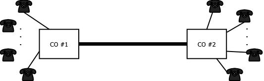
In addition to packet based networking technologies, we have studied TDM and optical circuit technologies. Some of the earliest work in queueing theory was associated with phone networks and was done by Erlang. Consider Figure 1 which shows two telephone central offices (COs) connected to customers telephones. The COs are connected via trunk (link) that has a finite capacity. The essence of the problem here is that customers on the different COs will decide to call a customer on the other CO at unpredictable times (make a request for trunk resources) and stay on the phone for an unpredictable amount of (holding) time. If there is no more capacity available on the trunk when a request comes in then the user would be blocked. In the early phone system trunk capacity was a very expensive resource hence one of the problems that Erlang tackled was to understand the nature of the requests and holding times from a statistical (probabilistic) point of view and then predict the probability that a customer request would be blocked based on the trunk capacity.

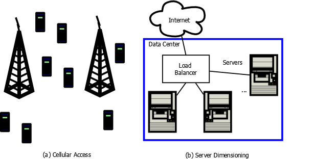
The telephony blocking concepts just mention naturally extend to high bandwidth TDM and optical networks with dynamic circuit setup and tear down. However, they are useful far beyond classic circuits. In Figure 2 we give two more modern examples. In (a) we show two cell towers (which have finite access capacity) and a multitude of cell phones that may want service, will use the service for an unpredictable amount of time, and may move from the region controlled by one base station to another. In (b) we show an application implemented in a data center that services requests from the Internet. The load balancer assigns requests to the servers based on their current load.

Beyond simple blocking behavior, one can also include queueing, i.e., a request could wait for an available server. Then the system modeler may also need to take into account balking behavior, where customers stuck in a queue get tired of waiting and leave the queue...

Congestion: Intuition

What causes packet delay in excess of propagation delay and switching time? What causes a blocking event, e.g., a cellular handoff failure not attributable to radio propagation problems? In both cases we have a shared costly resource. When a multitude of users attempts to use this resource at the same time this can cause congestion, resource exhaustion, or both. For example when going to the supermarket during busy hour you may encounter significant wait at the checkout counter. This is a type of congestion. When attempting to board a subway train during busy hour in Tokyo you may find the train is completely full, i.e., you are blocked. When attempting to see a new movie on a Friday night at 8PM you might wait in a long ticket line (queueing) only to find that all the seats have been sold (queueing and blocking).

Common queueing questions in networking:

1. How big should my packet buffer be on my nifty new SDN switch design?

2. How much delay will my packet experience as it traverses the network?

3. How many wavelengths do I need to turn up to keep the chance of blocking (wavelength collision) relatively low?

4. How many servers should I provision with my cloud provider to minimize the chances that a customer will not get serviced in a timely manner?

Queues (lines) can form even where there is plenty of bandwidth!

Example:

Consider a 100 sources sending constant bit rate traffic (say video) over Ethernet. Suppose that the Ethernet frame sizes are near the MTU, for example 1250 bytes = 10,000bits. If the sources have an average bit rate of 5Mbps per second they will send a packet every $1.0\times 10^4bits/5.0\times 10^6bps = 2mS$.

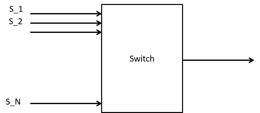
Suppose we have a 101 port Ethernet (1Gbps per port) switch with a server that is supposed to receive all these video streams as shown in Figure 3. How big or small could the output queue for this one port get?

To keep life easy let's assume a constant packet size of 10,000bits. How long does it take to transmit this on a 1Gbps port? Answer: $1.0\times 10^4 bits/1.0\times 10^9 bps = 1.0\times 10^{-5}s = 10\mu s$.

Since we have to send one of these packets every $2ms$, how many different streams can we send? Answer: $2ms/10\mu s = 2\times 10^{-3}/10\times 10^{-6} = 200$. Or we can think of each 1Gbps link having the equivalent of 200 packet arrival slots per 2ms.

Suppose every sender is very prompt and all are synchronized to send their packets at the same time. What will happen?

A packet queue will build up and drain away in a periodic manner as shown in Figure 4.

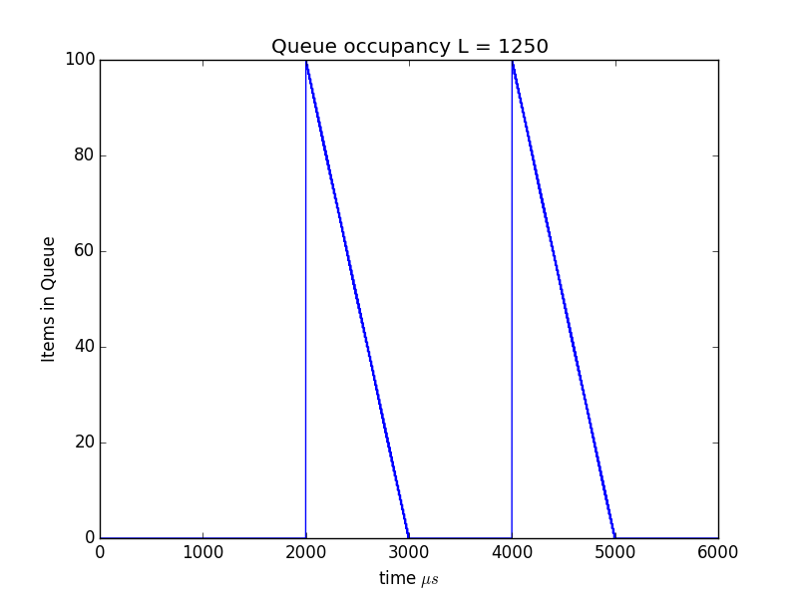
Important concepts: The average rate of the sources is 5Mbps but the peak rate of the source, i.e., the rate at which a packet is sent is 1Gbps.

Random Variables

A quick review of the rigorous roots of what we will be doing.

Basic Definitions

Definition In probability theory, the sample space, S, of an experiment or random trial is the set of all possible outcomes or results of that experiment. https://en.wikipedia.org/wiki/Sample_space

Networking examples:

1. {Working, Failed} state of an optical link

2. ${0,1,2,...}$ the number of requests to a webserver in any given 10 second interval.

3. $(0, \infty ]$ the time between packet arrivals at the input port of an Ethernet switch

Why care about the sample space? When we run simulations the values that we generate will be in the sample space. We will use both discrete and continuous as well as bounded and unbounded sample spaces.

Definition (Event) An event E is a subset of the sample space S.

Intuitively just a subset of possible outcomes.

Definition (Probability Measure) A probability measure P(A) is a function of events with the following properties:

1. For any event $A$, $P(A) \geq 0$

2. $P(S)=1$, ($S$ is the entire sample space)

3. If $A \cap B$ = $\emptyset$, then $P(A \cup B) = P(A) + P(B)$

Note that for infinite sample spaces we extend property 3 above to:

For any countable sequence of events $A_k$ that are pairwise disjoint, i.e., $A_i \cap A_j=\emptyset$, then $P(\cup_i A)= \sum_i P(A_i)$. See https://en.wikipedia.org/wiki/Probability_measure.

Some consequences:

• If $\bar A$ denotes the event consisting of all points not in A, then $P(\bar A ) = 1 - P(A)$.

• Example: The probability of a bit error occurring on a 10Gbps Ethernet link is $P(bit_error) =1.0\times 10^{-12}$ what is the probability that a bit error won't occur? $P(bit_good) = 1 P(bit_error) = 0.9999999999990$ (Twelve 9's).

• $P(\emptyset)=0$

Definition (conditional probability) Given two events A and B with $P(B) > 0$, then the conditional probability of $A$ given $B$ is defined as

$$P(A|B) = \frac{P(A\cap B)}{P(B)} \tag{CondProb}$$

Definition (independent events) Two events $A$ and $B$ are said to be independent if $P(A|B) = P(A)$.

A consequence of this is that if A and B are independent then $P(A \cap B) = P(A)P(B)$.

Example: consider a 1+1 fiber optic link where the lasers have a $1\times 10^{-3}$ probability of burning out in the next hour. What is the probability of link failure in the next hour if the lasers are "independent"? Let the failure of the first laser in the pair be event $A$, and the failure of the second laser in the pair be event $B$, then we want to know $P(A\cap B)$ assuming independence we find this by multiply the probabilities $P(A\cap B) = P(A)\cdot P(B)= 1\times 10^{-6}$.

Definition Probability Space A probability space consists of three parts:

1. A sample space, $S$ , which is the set of all possible outcomes.

2. A set of events $\scriptstyle \mathcal{F}$, where each event is a set containing zero or more outcomes.

3. The assignment of probabilities to the events via a probability measure $P$.

Definition Random Variable A random variable $X$ is a real valued function on the sample space, i.e., $X: S \rightarrow \mathbb{R}$.

We then can assign probabilities to ranges of $X$ values by using the probability measure on the events that correspond to the values in the range. For example:

The probability distribution for a random variable $X$ is defined by $P_X(x)=P(X=x)$.

The cumulative distribution function (CDF) for a random variable X is defined as ${F_X}(x) = P(X \leqslant x)$, and the complementary distribution function is defined as ${\bar F_X}(x) = P(X > x)$. Note from the fundamental properties of probabilities that ${\bar F_X}(x) + {F_X}(x) = 1$.

For a continuous random variable

$$p(x) = \frac{{d{F_X}(x)}}{{dx}} \tag{pdensity}$$

Moments

The n-th moments for discrete and continuous random variables are defined by:

$$E[{X^n}] = \sum\limits_k {{k^n}{P_X}(k)} \tag{MomentDiscrete}$$

and

$$E[{X^n}] = \int\limits_{ - \infty }^\infty {{x^n}{f_X}(x)dx} \tag{MomentCont}$$

respectively.

The first moment is known as the mean.

The variance is defined as $Var[X] = E[{(X - E[X])^2}]$

Multiple Random Variables

If we have multiple random variables, ${X_1},{X_2}, \ldots ,{X_n}$, defined on the same sample space $S$ we can ask what is the probability that their values lie in a particular range, e.g., a joint cumulative distribution function:

$${F_{{X_1},{X_2}, \ldots ,{X_n}}}({x_1},{x_2}, \ldots ,{x_n}) \equiv P({X_1} \leq {x_1},{X_2} \leq {x_2}, \ldots ,{X_n} \leq {x_n})$$

where $$P({X_1} \leq {x_1},{X_2} \leq {x_2}, \ldots ,{X_n} \leq {x_n}) \equiv P({X_1} \leq {x_1} \cap {X_2} \leq {x_2} \cap \ldots \cap {X_n} \leq {x_n})$$

As for events we can also define conditional probabilities and independence for random variables. In the discrete case we have:

$${P_{X|Y}}(x|y) = P(X = x|Y = y) = \frac{{P(X = x,Y = y)}}{{P(Y = y)}}$$

Independence of random variables relates back to independence of events and we have $${P_{X|Y}}(x|y) = {P_X}(x)$$ and $$P_{X,Y}(x,y) = P_X(x)P_Y(y)$$ as the definition and consequence of the independence of two random variables X and Y.

Note that we frequently make assumptions about the independence of random variables. In simulations our random number generators produce values that are designed to mimic a sequence independent identically distributed random variables. Note that it is a fundamental theorem that if X and Y are independent random variables then $$E[XY] = E[X]E[Y] \tag{IndMean}$$

Discrete Distribution Summary

• Bernoulli Distribution
  • Sample space {0, 1} or any two distinct values.
  • $P(X=1)=p$, $P(X=0)=1-p$
  • Models two outcome events
  • Most famous example: coin tosses
  • Mean: $p$, Variance: $p(1-p)$
  • Simulated in Python with from scipy.stats import bernoulli
• Geometric Distribution
  • Sample space either ${0, 1, 2, \ldots }$ or ${1, 2, 3, \ldots }$
  • Interpretation: the number of Bernoulli trials until an "event". I say event rather than "sucess" since the event may be a "link failure" or a bit error which no one really should consider a "sucess".
  • Networking example: how long do we wait the next bit error on a link.
  • Distribution: $Pr(X = k) = (1-p)^{k-1}p$
  • Mean: $1/p$, Variance: $\frac{1-p}{p^2}$
  • Simulate in Python with from scipy.stats import geom
• Binomial Distribution
  • Number of events in $n$ trials of independent (Bernoulli) trials with probability for an event $p$.
  • Sample space ${0,1,2, \ldots, n }$
  • Distribution: $Pr(X = k) = \binom n k p^k(1-p)^{n-k}$, for $k = 0, 1, 2, \ldots, n$ where $\binom n k =\frac{n!}{k!(n-k)!}$.
  • Mean: $np$, Variance: $np(1-p)$
  • Simulate in Python with from scipy.stats import binom.
• Poisson Distribution
  • Sample space: ${ 0, 1, 2, 3, ... }$
  • "expresses the probability of a given number of events occurring in a fixed interval of time and/or space if these events occur with a known average rate and independently of the time since the last event."
  • "The Poisson distribution can be derived as a limiting case to the binomial distribution as the number of trials goes to infinity and the expected number of successes remains fixed."
  • Parameter: $\lambda > 0$
  • Distribution: $P(X=k) = \frac{\lambda^k}{k!} e^{-\lambda}$
  • Mean: $\lambda$, variance: $\lambda$
  • Simulate in Python with from scipy.stats import poisson

Continuous Distribution Summary

• Exponential Distribution
  • We'll be using this to model the time (continuous) between events such as packet arrivals or servicing times. It has the very important "memoryless property"
  • Sample space: $x \in [0, \infty)$
  • Probabiliy density function: $p(x) = \lambda e^{-\lambda x}$
  • Mean: $1/\lambda$, Variance: $1/\lambda^2$
  • To simulate in Python from the standard library use from random import expovariate, from SciPy use from scipy.stats import expon note that the SciPy expon takes a scale parameter which is $1/\lambda$. Also note that lambda is a key work in Python and can't be used to describe the parameter of the exponential distribution.

Generating Random Samples with Python

There are three common Python libraries that provide psuedo random number generation with prescribed distribution functions.

• The Python standard library's random module
  • Features random bits, random integers, and random floats with a limited set of distribution functions.
• Numpy's random module
  • Numpy is a numerical computing package emphasizing array processing.
  • It contain a much larger collection of distributions than that found in Python's standard library and these are "array friendly". These are a subset of the available distributions in SciPy.
• SciPy's stats module
  • This library contains a huge number of continuous and discrete distributions.
  • Provides base classes for discrete and continuous that can be extended to create custom distributions.

Example 1 Uniform random numbers from the standard library.

import random
print(random.random()) # print the value of a single sample
x = [random.random() for i in xrange(10)]  # Produce a list of random values
print(x)  # print the list of random values
print('Average of x = {}'.format(sum(x)/float(len(x))))

Example 2 Exponential random numbers from the standard library

import random
print(random.expovariate(0.25)) # print one sample exponential with lambda = 0.25
xe = [random.expovariate(0.25) for i in xrange(10000)]  # Generate a lot of samples
print(xe[-5:]) # Print the last five of the samples
print('Average of xe = {}'.format(sum(xe)/float(len(xe))))  # Check against theory mean

Example 3 Binomial distributed random numbers from Numpy

from numpy.random import binomial
print(binomial(30, 0.1))  # Binomial sample n = 30, p = 0.1
xb = binomial(30, 0.1, size=10000)  # Don't have to use list stuff, Numpy likes arrays!
print(xb[:5])  # Look at first five entries
print('Average of xb = {}'.format(sum(xb)/float(len(xb))))

Example 4 Bernoulli distributed random numbers from SciPy

from scipy.stats import bernoulli
myrv = bernoulli(p=0.14) # Create a Bernoulli object with fixed p = 0.14
print(myrv.rvs()) # Generate and print a sample
xbern = myrv.rvs(size=10000)  # Generate a big array
print(xbern[:10]) # look at the first 10
print(sum(xbern)) # look at the sum
print('Average xbern = {}'.format(sum(xbern)/float(len(xbern)))) # compute the average.

Memoryless Property of Distributions

A more subtle property of a distribution that is reminiscent but not the same as independence is the memoryless property. Random variables with this property are much more amenable to analysis.

Definition A continuous random variable, X, defined on $[0,\infty )$ is said to be memoryless if given $s, t \ge 0$

$$P(X > t + s| X > t) = P(X > s) \tag{mLessCont}$$

Definition A discrete random variable, X, is said to be memoryless if given $n, m \ge 0$ $$P(X > m + n|X > m) = P(X > n) \tag{mLessDis}$$

Compared to independence: https://math.stackexchange.com/questions/200344/relation-between-memorylessness-and-independence.

This is not the same as saying that these events are independent! How would we change the above equation for independence?

Facts:

1. The only continuous memoryless distribution is the exponential distribution.

2. The only memoryless discrete distribution is the geometric distribution

Example: verify the memoryless property of exponential distributions

As some practice with probabilities and such let's verify that the exponential distribution has the memoryless property. First lets look at the conditional probability in the definition of memoryless property: $$P(X> t+s | X > t) \equiv \frac{P(X > t+s \cap X > t)}{P(X > t)}$$ Now $[t+s, \infty) \cap [t, \infty) = [t+s, \infty)$ since $s,t \ge 0$ so $$P(X > t+s \cap X > t)=P(X > t+s)$$ using this in our conditional probability definition (CondProb) gives: $$P(X> t+s | X > t) = \frac{P(X>s+t)}{P(X > t)}$$ Now combining this with our the memoryless property, equation (mLessCont), gives: $$P(X> s) = \frac{P(X>s+t)}{P(X > t)}$$ which yields: $$P(X > s)P(X > t) = P(X>s+t) \tag{mem2}$$

This alternative form of the memoryless property is highly suggestive of an exponential function. Let's compute $P(X>y)$ for $y > 0$ given that y is exponentially distributed:

$$P(X>y) = \int_y^\infty \lambda e^{-\lambda x}dx=e^{-\lambda y}$$ To complete our check we use $P(X>y)=e^{-\lambda y}$ in equation (mem2) to get: $$e^{-\lambda s}e^{-\lambda t} = e^{-\lambda (s+t)}$$

Measurement Techniques

Periodic sampling can have trouble discovering periodic phenomena. Periodic sampling is also subject to manipulation. An alternative is random sampling. In particular sampling with exponentially distributed inter-arrival times (as a result of the memoryless property) can provide unpredictable and unbiased samples (see sections 11.1 and 11.2 of RFC2330). This technique is called Poisson sampling.

Example: One-way Delay Metric for IP (http://tools.ietf.org/html/rfc2679)

A single measurement is defined fairly precisely:

1. Source and Destination must have synchronized clocks.

2. NTP can get down to low millisecond accuracy with careful work and good servers.

3. GPS can get down to 10 of microsecond accuracy.

4. Source puts a time stamp for the transmit time into the packet

5. Receiver notes the reception time upon packet inspection and derives the one way delay.

A Poisson sampled stream of these measurements can be defined and various statistics of the stream can be determined such as: Percentiles, Median, Minimum, etc... Note in some cases a "geometric" sampling methodology will be appropriate. Such a technique is hinted at in the sFlow specification (http://sflow.org/sflow_version_5.txt).

Discrete Event Simulation

Network performance evaluation via simulation consists of the processes of modeling, evaluation, and interpretation of results. Network simulation differs from network emulation. In network emulation, i.e., with an emulator such as Mininet, complete networking data and control planes are used. For example full Ethernet, IP, and upper layer content will be contained in packets which will be forwarded by full functionality switches that happen to be implemented in software.

As compared to emulation or network testbeds based on real hardware network simulations are based on simplified models of network functionality. Such simplified models permit:

• The evaluation of networking scenarios that would take too long to emulate.
• The evaluation of behavior not built into existing protocols/hardware.
• The evaluation of networking scenarios that are too large to emulate.

The key to developing network simulation models is determining what processes and attributes to include and what to discard. Extra details not relevant to answering the performance or behavioral question can result in longer and more expensive (computationally) simulation runs (evaluation). On the other hand insufficient detail in critical areas can result in worthless or misleading results.

The evaluation of networking simulation models is done with discrete event simulation (DES). In a discrete event simulation time advances in uneven steps as the simulator advances from each discrete event to the next. In the network simulations we will be performing, examples of events include:

• The generation of a packet
• The arrival of a packet at a switch port
• The transmission of a packet from a switch port
• A request arriving at a server
• The dispatch of a response from a server

In discrete event simulation it is the job of the simulator to run (evaluate) the network model over a given interval of simulated time or a prescribed number of events. Examples of open source (and partially open source) network oriented and general purposed discrete event simulators include:

• SimPy is a native Python general purpose simulator which we will be using to build our simple network simulator.
  • Works with all modern Python distributions
  • Relatively small size, i.e. less than 0.5MB installed with Python.
• OMNeT++ "OMNeT++ is an extensible, modular, component-based C++ simulation library and framework, primarily for building network simulators."
  • Contains very nice visualization tools to aid in understanding of network protocols and debugging of simulation models. Ajustable simulation rate during visualization.
  • Extensive networking protocol libraries (Ethernet, IP, MPLS, control planes, etc...)
  • Uses a special language on top of C++ to build network models from components.
  • Fairly large size, compressed download ~ 475MB. Runs on Windows and Linux.
• ns-3 "ns-3 is a discrete-event network simulator for Internet systems, targeted primarily for research and educational use."
  • Key Technologies: "ns-3 is a C++ library which provides a set of network simulation models implemented as C++ objects and wrapped through python. Users normally interact with this library by writing a C++ or a python application which instantiates a set of simulation models to set up the simulation scenario of interest, enters the simulation mainloop, and exits when the simulation is completed."
  • "The ns-3 simulation core supports research on both IP and non-IP based networks. However, the large majority of its users focuses on wireless/IP simulations which involve models for Wi-Fi, WiMAX, or LTE for layers 1 and 2 and a variety of static or dynamic routing protocols such as OLSR and AODV for IP-based applications."
  • Supports very detailed models and can function as a network emulator. No visualization or IDE tools. Source tarball size is about 24MB. Run on Linux.

Discrete Event Simulation with SimPy

We'll be doing simulations directly in Python via the Simpy external package. You'll need to install this in addition to your python distribution, e.g., pip install simpy. Note that Simpy should not be confused with the nice symbolic math package Sympy.

The SymPy documentation describes itself as a process oriented simulation. This has nothing to do with operating system processes! It means that we model many of the entities in our network as an "active" entity. It is the job of the simulator to coordinate which of these active entities gets to run next based on simulated time and the list of pending events. SimPy makes use of Python generators. This is a very deep and interesting computer science topic that we will not have time to cover in any depth. For a good tutorial on python coroutines see this PDF. We'll think of python generators as "mini-processes" that yield (stop) themselves and can be resumed with possibly new inputs. Here is a simple example (try this at a python command line):

def inc3():   # Looks like a regular function BUT it isn't!!!
    i = 3
    while True:  # Look like an infinite look but it isn't!!!
        yield i  # This statment suspends the generator and returns a value
        i += 3   # We resume here if the generator is called again

Although the above looks like a function definition it is not!!! The presence of the yield Python keyword turns this into the definition of a generator function. We then use the generator function to create generator objects. We then run the generator objects with their next method.

tmp1 = inc3() # create a generator object
tmp2 = inc3() # create another generator object
print(tmp1.next()) # run the first object
print(tmp1.next()) # run the first object
print(tmp1.next()) # run the first object
print(tmp2.next()) # run the 2nd object, note that it keeps it own state!

In addition to receiving values from a generator object we can send values into a generator as in the following somewhat silly example (try this at a python command line):

def silly(): # Not a reqular function since it contains a yield statement
    n = 1
    while True:
        name = (yield n)  # Yields the value of n, but assigns to name whatever is sent
        print (n*(name + " ")) # Prints the name sent n times
        n += 1

tmp = silly() # creates the "silly" generator object
tmp.next()  # Runs the generator to the yield point and gets the value
tmp.send("EE283") # Sends in a value and gets the yielded value
tmp.send("SJSU!")
tmp.send("EE283!")

This ability to start, stop, and resume code running in separate objects is extremely powerful and forms the basis of discrete event simulation with SimPy. At a minimum one needs the notion of simulated time and a simulator object to run the simulated processes at the appropriate time.

Let's look at a very simple simulation of two clocks that tick at different rates. The SimPy implementation uses the following code (try this at the python command line):

import simpy
def clock(env, name, tick): # First argument is the simulation environment
    while True:
        print(name, env.now)
        yield env.timeout(tick) # Generator function

env = simpy.Environment() # creates the simulator
env.process(clock(env, 'fast', 0.5)) # create clocks, wraps them in a "process",
env.process(clock(env, 'slow', 1.0)) # and add to the simulator
env.run(until=2) # run simulation till time = 2.

Modeling Network Packet Delay and Loss

Given the SimPy simulation infrastructure we will add a minimal set of classes to allow us to model packet delays and losses in a network. The basic classes include:

• Packet: Our packet model will be minimalistic and general at the same time.
  1. We will not care about the details of IP, Ethernet, or MPLS packets, but will model a general variable sized packet. We will use a parameter to indicate the packet size but not have our packet contain any actual content.
  2. We will include source, destination, a flow identifier, and a packet identifier but no other common packet header data. These fields may or may not be needed in a given simulation.
  3. Since one of our main performance criteria we are seeking to measure is delay we will include in our packet the simulated time that it was created. Note that this is the first case we've added something to our model to aid in obtaining information from our simulations.
• Packet Generator: Although packets are generated by application protocols in response to user actions we will not be modeling user behavior or higher layer protocols. Instead we will be modeling the raw generation of packets. A PacketGenerator object will be created with the following parameters and state:
  1. The "inter-arrival" time distribution. This is a function that generates values that represent the time between the generation of packets.
  2. The packet size distribution. This is a function that generates values for the size of the packets generated.
  3. Each packet generator can have an identifier and a flow identifier that gets put into the generated packet.
  4. Each packet generator will keep track of the number of packets that it has sent.
  5. The packet generator has an "output port", i.e., reference to an object that it will send the packet to.
• PacketSink: An endpoint for packets after they have traversed our simulated network. Although one might think that there isn't anything to be done here, this is where we will keep track of some key performance information:
  • On packet arrival we will record the packet waiting time (delay) based on the generation time in the packet object and the current simulation time.
  • If desired we will separately record the time the packet arrived at the sink. We'll use this to see what the arrival process looks like statistically.
• SwitchPort: At this time we will not model an entire switch data plane but only a switch output queue and port. We allow an arbitrary number of inputs to our switch port model. The switch port is modelled with the following parameters and state:
  • A queue that contains packets. This can have finite or infinite capacity.
  • A rate for the link that corresponds to the switch port. We do not separately model the link.
  • We track the number of packets received and dropped, the queue size in packets and bytes, and whether the output port is currently busy sending a packet.
  • Another element sends a packet to a switch port via a put(packet) method.
• PortMonitor: This class can be used to monitor the distribution of the queue size in a SwitchPort object over time. It it modelled by the following parameters and state:
  • A list of sizes.
  • A function that provides the time between when samples of the queue size should be taken. If set to an exponential random distribution we get Poisson sampling.
  • An indicator as to whether we are interested in the number of objects or the number of bytes in the switch port queue.

A UML diagram of these classes is shown in Figure 5 and the source Python code SimComponents.py.

Example 1: Two packet sources and a sink

Simple example of PacketGenerator and PacketSink from the SimComponents module. Creates two constant rate packet generators and wires them to one sink.

from random import expovariate
import simpy
from SimComponents import PacketGenerator, PacketSink

def constArrival():  # Constant arrival distribution for generator 1
    return 1.5

def constArrival2():
    return 2.0

def distSize():  # Will make packet sizes random
    return expovariate(0.01)

env = simpy.Environment()  # Create the SimPy environment
 # Create the packet generators and sink
ps = PacketSink(env, debug=True)  # debugging enabled so we can see arrivals
pg = PacketGenerator(env, "EE283", constArrival, distSize)
pg2 = PacketGenerator(env, "SJSU", constArrival2, distSize)
 # Wire packet generators and sink together
pg.out = ps
pg2.out = ps
env.run(until=20) # Run it

Example 2: An overloaded output port

Simple example of PacketGenerator, SwitchPort, and PacketSink from the SimComponents module. Creates a constant rate packet generator, connects it to a slow switch port, and then connects the switch port to a sink. The queue size is made small an the port speed slow to verify packet drops.

import simpy
from SimComponents import PacketGenerator, PacketSink, SwitchPort

def constArrival():
    return 1.5    # time interval in seconds

def constSize():
    return 100.0  # bytes

env = simpy.Environment()  # Create the SimPy environment
 # Create the packet generator and sink
ps = PacketSink(env, debug=True)
pg = PacketGenerator(env, "SJSU", constArrival, constSize)
switch_port = SwitchPort(env, rate=200.0, qlimit=300)
 # Wire packet generators and sinks together
pg.out = switch_port
switch_port.out = ps
 # Run it
env.run(until=20)
print "waits: {}".format(ps.waits)
print "received: {}, dropped {}, sent {}".format(ps.packets_rec, switch_port.packets_drop, pg.packets_sent)

Output:

id: 1, src: SJSU, time: 1.5, size: 100.0
id: 2, src: SJSU, time: 3.0, size: 100.0
id: 3, src: SJSU, time: 4.5, size: 100.0
id: 4, src: SJSU, time: 6.0, size: 100.0
waits: [4.0, 6.5, 9.0, 11.5]
received: 4, dropped 6, sent 13

Example 3: Synchronized CBR sources

With this background we can now understand how the example in the Congestion: Intuition section can be simulated and the queue sizes plotted over time. Below we show use of SimComponents to simulate a lot of synchronized constant bit rate sources. This example is set up so one can vary the packet size and see the effects on worst case queue size and delay. Change the L value for bytes per packet. Also in the packet monitor change the count_bytes settings between True/False to go between packet count and byte count in the queue.

import simpy
import matplotlib.pyplot as plt
from SimComponents import PacketGenerator, PacketSink, SwitchPort, PortMonitor

N = 100     # Number of sources
r = 5.0     # average source rate is 5Mbps
C = 1000.0  # Port rate is 1Gbps
L = 1250    # bytes per packet
packet_time = 8*L/r  # in micro seconds
print "inter-packet arrival time = {} in micro seconds".format(packet_time)

def cbr_dist():
    return packet_time

def size_dist():
    return L

def samp_dist():
    return 1.0

 # Create the SimPy environment. This is the thing that runs the simulation.
env = simpy.Environment()
 # Create the switch port and sink
ps = PacketSink(env, debug=False)
switch_port = SwitchPort(env, C)
 # Create N packet generators and wire to the switch port
pgs = []
for i in range(N):
    name = "pg{}".format(i)
    pg = PacketGenerator(env, name, cbr_dist, size_dist)
    pg.out = switch_port
    pgs.append(pg)
 # If you want to monitor any switch ports, use a PortMonitor.
pm = PortMonitor(env, switch_port, samp_dist, count_bytes=False)
 # switch port and sinks together
switch_port.out = ps
 # Run it
env.run(until=6000)  # Run time in micro seconds
print "Maximum wait = {} micro seconds".format(max(ps.waits))
print "Maximum queue size in bytes = {}".format(max(pm.sizes))
print "average system occupancy in bytes: {}".format(float(sum(pm.sizes))/len(pm.sizes))

fig, axis = plt.subplots()
axis.plot(pm.sizes)
axis.set_title("Queue occupancy L = {}".format(L))
axis.set_xlabel(r"time $\mu s$")
axis.set_ylabel("Items in Queue")
 # fig.savefig("CBRQueueItemsL{}.png".format(L))
plt.show()

Modeling Blocking with Multiple Servers

To model circuit switching blocking, cellular access blocking, or server access blocking we will need the following ingredients in our simulation:

• A request that utilizes circuit or server resources for an amount of time determined by a distribution and accompanying parameters.
• A request generator to model the arrival of requests to the set of resources. The inter-arrival time of the calls would need to be model.
• A finite capacity resource pool that represents the TDM time slots, optical wavelengths, cellular channels, or web servers.

With SymPy we can model the request process as follows. Currently this process uses exponentially distributed random samples for request service time.

def request_process(env, resource_pool, service_time):
    with resource_pool.request() as request:
        yield request # Requests resource from pool then holds it
        yield env.timeout(random.expovariate(1.0/service_time))

We use SymPy's Resource class to model our resource pool, however their Resource class includes a waiting queue if all resources are busy so we will need to check the count of resources in use and determine blocking in our code.

We model the request generator as follows. The request generator keeps request generation and blocking counts and currently uses exponentially distributed arrival time samples.

class RequestGenerator(object):
    def __init__(self, env, arrival_time, service_time, resource_pool):
        self.env = env
        self.resource_pool = resource_pool
        self.a_time = arrival_time
        self.s_time = service_time
        self.capacity = resource_pool.capacity
        self.request_count = 0
        self.requests_blocked = 0
        self.env.process(self.run())  # Add run() process to the simulation

    def run(self):
        while True:
            yield self.env.timeout(random.expovariate(1.0/self.a_time))
            self.request_count += 1
            if self.resource_pool.count == self.capacity:  # At capacity, call blocked!
                self.requests_blocked += 1
            else:  # create and start a new call process
                self.env.process(request_process(self.env, self.resource_pool, self.s_time))

Example main program using the previous generator function and class:

import random
import simpy
from erlang import erlangB

A = 17.0 * 1.3  # The offered load in Erlangs
k = 25  # The number of "server" or trunk resources
env = simpy.Environment()  # The simulation environment.
resource_pool = simpy.Resource(env, capacity=k)  # The "resource" pool
call_gen = RequestGenerator(env, 1.0/17.0, 1.3, resource_pool)
env.run(until=5000.0)
print 'Total calls = {}, Dropped calls = {}, Blocking Probability = {}'.\
    format(call_gen.request_count, call_gen.requests_blocked, float(call_gen.requests_blocked)/call_gen.request_count)
print 'Theoretical call blocking = {}'.format(erlangB(A, k))

Example output:

Total calls = 84816, Dropped calls = 7121, Blocking Probability = 0.0839582154311
Theoretical call blocking = 0.0859945456849

The complete Python code for this example CallBlocking.py, this also uses erlang.py to compute the theoretical probability that you will learn about in the next section.

Queueing Theory

To understand the systems of interest we need to deal with random behavior over time. This is the field of stochastic processes.

Stochastic Processes

Definition [Zukerman2013a] For a given index set T a stochastic process ${ X_t,t \in T }$ is an indexed collection of random variables. If $T$ is countable then we say that we have a discrete-time process, otherwise the process is a continuous time process.

Note that at this point we have not put any constraints on the $X_t$, i.e., we have not assumed that they are identical or independent, or have a particular distribution. Four combinations are generally studied:

Random Variable Type	Index Discrete	Index Continuous
Discrete	Discrete Time, Discrete Space	Continuous Time, Discrete Space
Continuous	Discrete Time, Continuous Space	Continuous Time, Continuous Space

Counting Processes

Example (A counting process) [Zukerman2013a]: suppose we have a sequence of arrivals that occur at random points in time (some call this a point process). Let $N(t)$ be the number of arrivals up to time $t$. Then we have:

1. $N(t) \geq 0$

2. $N(t)$ is an integer

3. if $s > t$, then $N(s) \geq N(t)$ and $N(s) – N(t)$ is the number of arrivals in $(t, s]$.

Note that $N(t)$ is not an independent process, i.e., the values of $N(t_1)$ and $N(t_2)$ for $t_1 \neq t_2$ are not independent random variables!

Example (Poisson Process): A counting process is said to be a Poisson process with rate $\lambda$ if

1. $N(0) = 0$

2. The process has “independent increments”, i.e., for $s > t > u > v$ the random variables $N(s)-N(t)$ and $N(u)-N(v)$ are independent (in words the number of arrivals in non-overlapping time periods are independent random variables)

3. The number of arrivals in an interval of length $t$ has a Poisson distribution with mean $\lambda t$.

Fact: The inter-arrival times of a Poisson process have an exponential distribution with parameter $\lambda$.

Kendall's Notation [Zukerman2013a]

Kendall's notation is a shortcut notation to describe queueing systems of various types. Key ingredients are the arrival process, service process, and the number of servers. Secondary ingredients are the buffer size and queueing discipline. We will look at queueing disciplines later, now we will always assume "first come first served" (also known as "first in first out").

{arrival process}/{service distribution}/{number of servers}/{buffer size}-{queue discipline}

Common symbols: M (Markovian - Poisson for the arrival process or Exponential for the service time distribution required by each customer), G (General), GI (General and independent), and Geom (Geometric).

Defaults: buffer size is infinite, Queueing discipline is FIFO.

G/G/1 Utilization [2] {#ref:RND24SFNjilHp#}

Very few analytic results are available for queueing systems with general arrival and departure distributions. We cover two important ones here. The first is concerned with the average amount of time that the server is busy. Denoted by $\hat U$.

Consider the G/G/1 queue. Arbitrary arrival process, arbitrary service times, infinite queue size.

Let $X_S$ be a random variable representing the service time and let $E[X_S] =1/\mu$ be the mean service time where $\mu$ is the service rate. Similarly let $X_A$ be a random variable representing the inter-arrival times and let $E[X_A]=1/\lambda$ be the mean inter-arrival time with $\lambda$ the arrival rate.

Lemma  $\hat U = \lambda / \mu$ if $\lambda / \mu < 1$.

Proof [Zukerman2013a]

Let $L$ be a long period of time, the average number of customers arriving in period $L$ will be $\lambda L$, the average number of customers served will be $\mu \hat U L$, since $L$ is large, and the queue is stable $\mu \hat UL = \lambda L$ and hence the result.

Corollary The probability that the G/G/1 queue is empty is $p_0 = 1 - \hat U = 1 - \lambda / \mu$.

Little's Formula

Let $Qnum(t)$ denote the number of customers (packets, whatever) in the system (in queue and in service), and $Delay(i)$ represent the delay for the i th customer including service time then

$$E[{Q_{num}}] = \lambda E[Delay]$$

Note that $Qnum(t)$ is a discrete space, continuous time process while Delay(i) is a continuous space, discrete-time process and the above formula relates the two. We'll only study how to get the probabilities for Q.

Proof Also See [Mir2007] or [Zukerman2013a]

Let $A(t)$ be the number of arrivals up to time $t$. Let $D(t)$ be the number of departures up to time $t$, then the number of number of items in the system $Q(t) = A(t) - D(t)$, for $t \geq 0$. Now $$E[Q] = \frac{1}{L} \int_0^L Q(t) dt$$ for $L$ a long period of time. Let $W_i$ be the waiting time of the i^th^ item. The key "trick" to proving Little's Formula comes down to looking at two ways of expressing the total time that all packets spend in the system. One way to compute this is: $$Time_{all , packets} = \int_0^L Q(t)dt $$ Another way of computing the total time spent by all packets in the system is to sum their individual waiting times: $$Time_{all , packets} = \sum_{i=1}^{A(L)} W_i $$ Equating these and dividing by $L$ gives: $$E[Q] = \frac{1}{L} \int_0^L Q(t) dt = \frac{1}{L} \sum_{i=1}^{A(L)} W_i$$ Now $\lambda = A(L)/L$ and $$E[Delay] = \frac{1}{A(L)} \sum_{i=1}^{A(L)} W_i$$ and then: $$E[Q] = \frac{1}{L} \int_0^L Q(t) dt = \frac{A(L)}{L}\frac{1}{A(L)} \sum_{i=1}^{A(L)} W_i$$ which finally gives: $$E[Q] = \lambda E[Delay]$$

Queueing Analysis

We now look at a number of queueing systems for which we can obtain more detailed analytical results. We restrict ourselves to continuous time Markov Processes and make an extremely useful simplifying assumption on state transitions.

Continuous Time Markov Chains

These are more general than a Poisson process but have a memoryless property for ease of analysis.

Definition (for our purposes here) A continuous time Markov process is a discrete space, continuous time random process whose time to change between states is exponentially distributed.

Note that the rate at which the process changes state can depend upon the state, i.e., the exponential parameter $\lambda$ can be state dependent.

There is a vast literature on Markov processes and they been found useful in many situations. We are going to use some key results on Markov processes to simplify our analysis of relatively simple queueing systems.

Birth-Death Processes (One thing at a time)

With Markov processes we restrict ourselves to a discrete state space which is useful for modeling the number of items in a system. Now we will make the additional assumption that items arrive and depart the system one at a time. This isn't too big an assumption since we can model any simultaneous events as separate arrivals or departures that occur as close in time as needed.

Our analytic study of queueing systems will be intuitive (rather than rigorous) and will be based on birth-death processes that are stable, i.e., reach a steady state. We make use of the following assumptions/facts:

• Markov processes have a discrete state space
• We'll use the number of items in the system to represent the state. Note that the "system" depends on the problem at hand and could be an output port on a switch, a distributed application running in a data center, a cellular base station, etc...
• Assume items arrive and depart the system one at a time (birth-death process). Note that "items" can be packets, server requests, restaurant customers, etc...
• State transitions are exponentially distributed and the rates can depend on the state (continuous time Markov process.)

We represent the system, its states, and state transitions by a diagram of the form shown in Figure 6. In the diagram "birth" (arrival) rates in a particular state are denoted by $\lambda_i$ and "death" (departure) rates are denoted by $\mu_i$, and the number inside the circles denotes the number of items in the system.

Our general analysis proceeds as follows:

1. We make a stability/equilibrium assumption that the probability $P_n$ of being in state $n$ is well defined. This would not hold, for example, if the system is being oversubscribed, i.e., requests are coming in faster than the service rate.

2. We intuitively talk of probability "balance" for states in our diagram (this notion can be made rigorous). For state $0$ if we equate the probability of leaving and entering the state we get: $$\lambda_0 P_0 = \mu_1 P_1 \tag{State0}$$

3. For a general state $n$ the balance equation would be: $$\lambda_{n-1} P_{n-1} + \mu_{n+1}P_{n+1} = \mu_n P_n + \lambda_n P_n \tag{StateN}$$

4. Let's look at the balance equation for state $1$: $$\lambda_{0} P_{0} + \mu_{2}P_{2} = \mu_1 P_1 + \lambda_1 P_1 \tag{State1}$$

substituting in from equation (State0) gives: $$\mu_{1} P_{1} + \mu_{2}P_{2} = \mu_1 P_1 + \lambda_1 P_1$$ which then simplifies to: $$\mu_{2}P_{2} = \lambda_1 P_1$$ 5. We can now establish a general relation via mathematical induction. We assume $\mu_nP_n = \lambda_{n-1}P_{n-1}$ (induction hypothesis) and show it is true for $n+1$. Starting the general balance equation: $$\lambda_{n-1} P_{n-1} + \mu_{n+1}P_{n+1} = \mu_n P_n + \lambda_n P_n$$ Substitue in the induction assumption: $$\mu_nP_n + \mu_{n+1}P_{n+1} = \mu_n P_n + \lambda_n P_n$$ Which gives $$\mu_{n+1}P_{n+1} = \lambda_n P_n \tag{GenRelation}$$ and we have proven the general relation.

6. Given we have established $P_n = \lambda_{n-1}/\mu_n P_{n-1}$, let $\rho_n = \lambda_{n-1}/\mu_n$ and we can write $P_n = \rho_n P_{n-1}$. Applying this expression starting from $P_0$ we get:

$$P_n = \left(\prod_{k=1}^n \rho_k \right)P_0 \tag{ProbN}$$

8. One last piece we need to remember before we analyze specific systems is that sum of the probabilities of being in a state must equal 1: $$\sum_{k=0}^\infty P_k = 1 \tag{Normalization}$$

M/M/1 Queue

Now consider a single server queueing system with Exponential inter-arrival rate $\lambda$, and Exponential service times with rate $\mu$, with infinite storage capacity. The state transition diagram would simplify to Figure 7.

We then have $\rho_n =\lambda/\mu \equiv \rho$ for all $n$ and from our general Birth-Death result equation (ProbN) $$P_n = \rho^nP_0$$ Our basic probability condition equation (Normalization) requires: $$\sum_{n=0}^\infty P_n = 1 = \sum_{n=0}^\infty \rho^n P_0$$ This gives $$P_0 = \frac{1}{\sum_{n=0}^\infty \rho^n}$$ Recall, or look up, or derive it yourself: $$S_N = \sum_{n=0}^N \rho^n = \frac{1-\rho^{N+1}}{1-\rho} \tag{GeoSum}$$

and if $0 < \rho < 1$ we have $$\lim_{N \to \infty} S_N = \frac{1}{1-\rho}$$ So we get the probability of the system being empty is $$P_0 = 1-\rho $$ which corresponds to our G/G/1 utilization result, but now we also have the probability to find $n$ packets (items) in the system: $$P_n = \rho^n(1-\rho ) \tag{MM1Prob}$$

To find the average number of items in the system we compute the mean: $$E[Q] = \sum_{n=0}^\infty n P_n = \sum_{n=0}^\infty n \rho^n(1-\rho ) $$ pulling out the $(1-\rho)$ gives: $$E[Q] = (1-\rho )\sum_{n=0}^\infty n \rho^n $$ Look up (or use a derivative on infinte sum $S$): $$\sum_{n=0}^\infty n \rho^n = \frac{\rho}{(1-\rho)^2}$$ Using this in the previous expression gives us: $$E[Q] = (1-\rho ) \frac{\rho}{(1-\rho)^2} = \frac{\rho}{(1-\rho)} \tag{MM1Queue}$$

Recall that $\rho$ is the system "utilization". Based on this result can we ever have 100% utilization of a packet switching link?

But what is the average packet delay? The delay is a continuous space stochastic process and we don't know how to handle those, but we have Little's formula $E[Q] = \lambda E[D]$. This gives us:

$$E[D] = \frac{1}{\lambda}E[Q]=\frac{1}{\lambda}\frac{\rho}{(1-\rho)}$$

Using $\rho = \lambda/\mu$ gives: $$E[D] = \frac{1}{\mu(1-\rho)} \tag{MM1Delay}$$

What happens to the queue size as the utilization nears 100%? Note to web readers: at this point in the course I would have students use discrete event simulation to simulate a switch output port with exponential packet inter-arrival times and exponentially distributed packet sizes (to give exponential service times) and verify the probability distribution, mean queue size, and average packet delay that we just derived. See my mini course on Basic Network Simulations in Python for code samples.

Finite Buffers: M/M/1/k

Let's look at a system with finite buffers to gain some insight into packet loss due to buffer overflow. The main thing to notice about the system shown in Figure 8 is that it is finite, i.e., does not continue forever to the right.

The balance equations are the same as the M/M/1 case: $$P_n = \rho^n P_0$$ with $\rho = \lambda/ \mu$. However the normalization condition is different due to the finite number of states: $$\sum_{n=0}^k P_n = 1 = \sum_{n=0}^k \rho^n P_0$$ Using our geometric sum formula (GeoSum): $$P_0 \frac{1- \rho^{k+1}}{1-\rho} = 1$$ which gives: $$P_0 = \frac{1-\rho}{1- \rho^{k+1}}$$ and hence $$P_n = \frac{(1-\rho)\rho^n}{(1- \rho^{k+1})}$$

The formula for mean number of items in the system gets somewhat messy and can be found in here for those interested. What is more interesting is the probability of packet loss. This will be the same as the probabiliy of a packet arriving at the system to find it full ($n=k$): $$P_k = \frac{(1-\rho)\rho^k}{(1- \rho^{k+1})} \tag{MM1kLoss}$$

Multiple Servers with no waiting space: M/M/k/k

A multiple server system with no waiting space can be used to model blocking in circuit switching, cellular access, amongst other situations. The key change from an M/M/1 or M/M/1/k system is that the service rate varies with the state the system is in. Suppose servers are identical with individual service rate $\mu$, if we are in a state with $m$ active servers then the rate that we would leave that state is $m\mu$. This leads to the state transition diagram of Figure 9 for a system with $k$ servers and no waiting space.

Let $A = \lambda / \mu$ then $$\rho_n = \frac{\lambda_{n-1}}{\mu_n} = \frac{\lambda}{n\mu}$$ We calculate the probabilities: $$P_n = P_0 \prod_{j=1}^n\rho_j = P_0 \prod_{j=1}^n \frac{\lambda}{j\mu} = \frac{A^n}{n!}P_0$$ for $1 \leq n \leq k$. The normalization condition $\sum_{n=0}^k P_n = 1$ gives: $$P_0 \sum_{n=0}^k \frac{A^n}{n!} = 1$$ so $$P_0 = \frac{1}{\sum_{n=0}^k\frac{A^n}{n!} }$$ The probability of being blocked is the same as the probability of finding all $k$ servers in use and is known as the Erlang B formula $E_k(A)$: $$E_k(A) \equiv P_k = \frac{\frac{A^k}{k!}}{\sum_{n=0}^k\frac{A^n}{n!} } $$

Note that in the multiple server case $A$ maybe greater than one! In Figure 10 we show a plot of the Erlang B formula for 24 servers as the load varies:

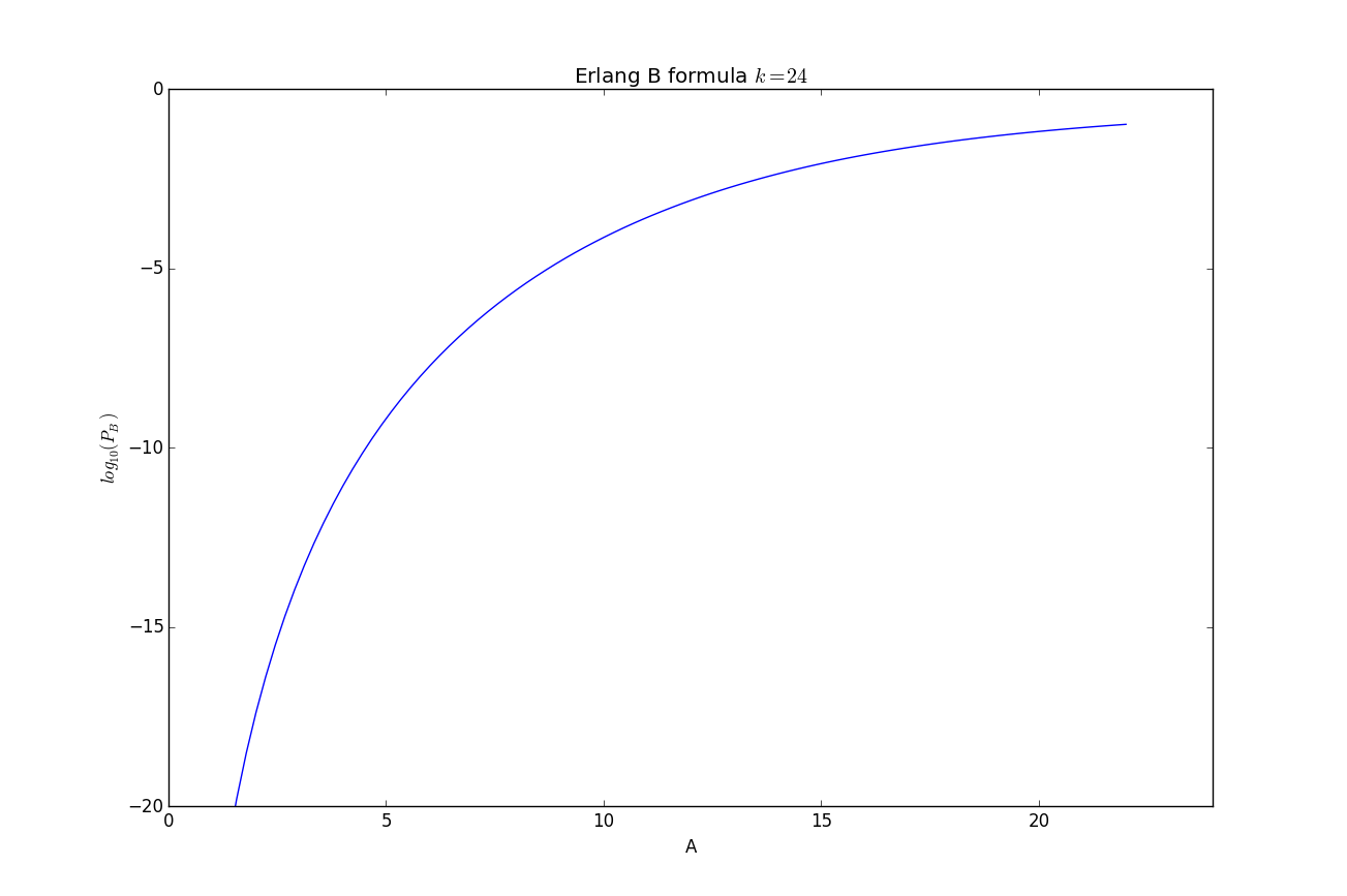
The Erlang B formula as given above is not computationally friendly, for better ways to evaluate this function see Wikipedia, [Zukerman2013a], or my tiny erlang.py file.

Networks of Queues

We have learned to simulate fairly general networking scenarios, but so far we have only learned to analyze a few fundamental queueing systems. With the aid of some key theorems we will be able to extend our previous analytic queueing results to networks of queues and hence to models of real networks. This will provide us with an important mechanism to check our simulations.

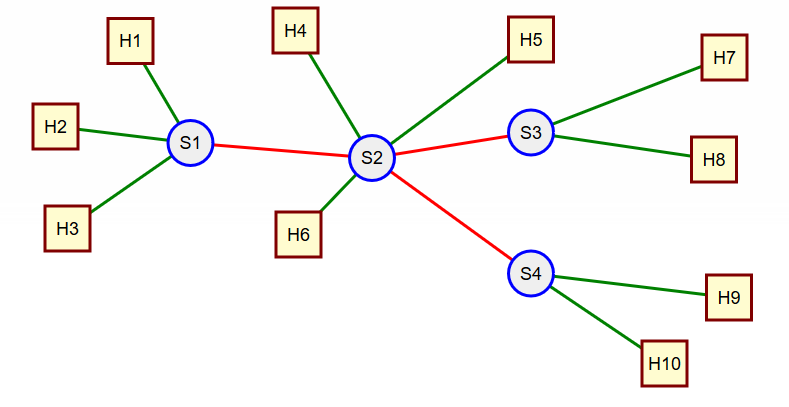
In the network shown in Figure 11 we are interested in load and queues that will build up on the network links shown in red, i.e., (S1, S2), (S2, S3), (S2, S4). We will, for simplicity, be interested only in traffic flowing from left to right on the links shown. We assume that all links shown on the left of a switch may send traffic to those links on the right but not the other way around.

With this assumption H1, H2, and H3 will all contribute traffic to link (S1, S2). What if anything can we say about the properties for the total traffic for link (S1, S2)? Suppose that we can model the traffic from each of the hosts as a Poisson process (exponential interarrival times), then we can make use of the following:

Definition [Zukerman2013a] A superposition of a number of Poisson processes is another point process that comprises all the points of the different processes.

Important property of the Poisson process [Zukerman2013a] is that the superposition of two Poisson processes with parameters $\lambda_1$ and $\lambda_2$ is a Poisson process with parameter $\lambda_1 + \lambda_2$.

Hence the load on the link (S1, S2) will be Poisson with rate $\lambda_1 + \lambda_2 + \lambda_3$. Now we are ready to look at the traffic entering switch S2. We assumed all host traffic was Poisson so we "understand" the traffic from H4 and H6, but what does the traffic on the link (S1, S2) look like? For that we need:

Burkes' Theorem [Zukerman2013a]

"in steady-state, the output (departure) process of M/M/1, M/M/k or M/M/${\infty}$ queue follows a Poisson process. Because no traffic is lost in such queues, the arrival rate must be equal to the departure rate, then any M/M/1, M/M/k, or M/M/${\infty}$ queue with arrival rate of $\lambda$ will have a Poisson departure process with rate $\lambda$ in steady-state."

Note how the input process must be Poisson and that the queues have infinite capacity. In addition we have the constraint of exponentially distributed service times. To realize this contraint in a packet switching scenario we must assume that all sources have the same exponential size distribution (with the same parameter $\lambda$).

At this point we would be able to analyze the output queue on switch S2 except that we have three output links (S2, H5), (S2, S3), (S2, S4) so we need more information for our analysis. In particular we need to know, at least probabilistically, which output ports on switch S2 the input ports send traffic to. In particular we could model forwarding and queueing in S2 in the way shown in Figure 12.

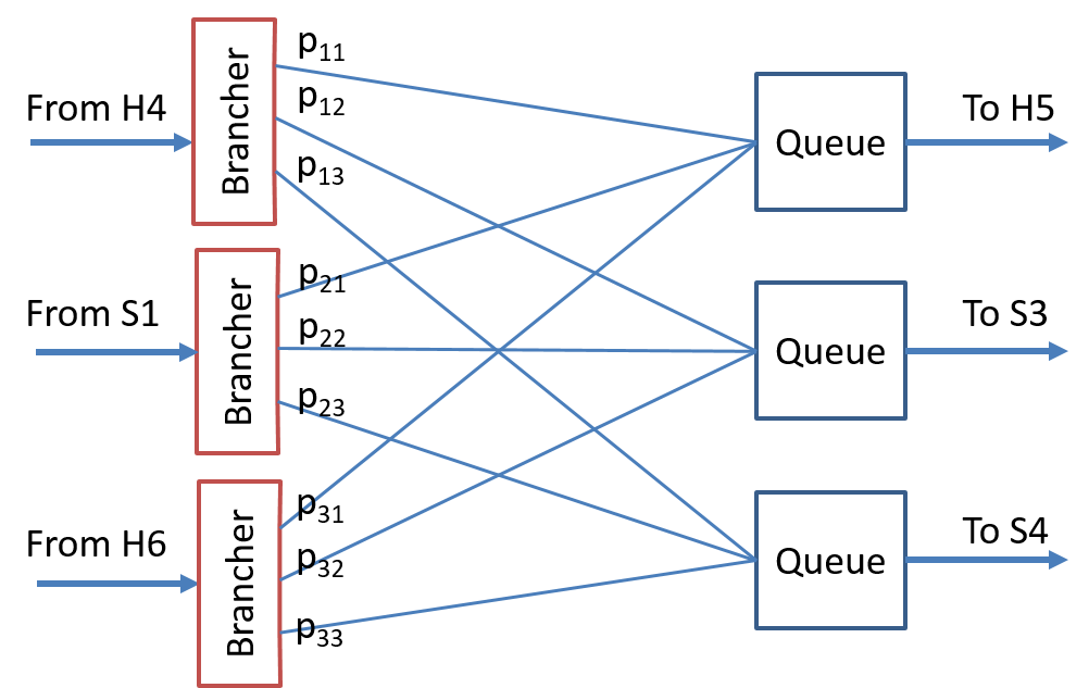
Note that no detailed routing/forwarding information is assumed just the probabilities that a packet will egress a particular port. With this additional information we can now make use of the following result:

Branching or Decomposition of a Poisson process [Trivedi1982]

Here we assume that a Poisson process with mean arrival rate $\lambda$ branches out into $n$ output paths. Assume that the selection of output path $i$ has probability $p_i$ $(1 \leq i \leq n)$ where $$\sum\limits_{i = 1}^n {{p_i}} = 1$$ Let ${ N(t)|t \geq 0 }$ be the input Poisson process and let ${ N_k(t)|t \geq 0 }$ for $1 \leq k \leq n$ denote the output processes. Then the conditional distribution of $N_k(t)$ given $N(t) = m$ is the multinomial distribution. In addition the random variables ${N_1}(t),{N_2}(t), \ldots ,{N_n}(t)$ are mutually independent and have Poisson distributions with respective parameters $p_1 \lambda ,p_2 \lambda , \ldots , p_n \lambda$.

For example a large link into a data center has a combined arrival rate of lambda and the different packets want to go to $n$ different places within the data center with differing probabilities, then we can still use nice Poisson models with modified arrival rates.

This result does not apply when packets are dropped when no room is available in a queue (known as "tail drop"). An alternate technique for dealing with buffer (queue) over flow is "random early detection" (RED) which randomly selects a packet in the queue to be dropped and hence can be analyzed as a random branch.

Analysis of links (S1,S2) and (S2, S3) Assume that the service rate on link (S1, S2) is $\mu_1$ and that on (S2, S3) is $\mu_2$ and that the branching probabilies at switch S2 are $p_{i,j}$ where $i = 1, 2, 3$ denotes the ingress links (H4, S2), (S1, S2), and (H6, S2) respectively and $j = 1,2,3$ denotes the egress links (S2, H5), (S2, S3), and (S2, S4) respectively.

The arrival rate for the queue for link (S1, S2) is just $\lambda_{Q1} = \lambda_1 + \lambda_2 + \lambda_3$. The utilization parameter is $\rho_{Q1} = \lambda_{Q1}/\mu_1$ from these we can obtain the average queue size and delay from the formulas for M/M/1 queues and Little's formula.

To compute the arrival rate from the queue for link (S2, S3) we use Burkes theorem and the branching result to give us: $$\lambda_{Q2} = p_{1,2}\lambda_4 + p_{2,2}\lambda_{Q1} + p_{3,2}\lambda_6$$ We then get the utilization parameter $\rho_{Q2} = \lambda_{Q2}/\mu_2$ and can use this to obtain average queue sizes and delays. Note that that average delay seen by a particular flow is the sum of the average delays at each queue it will have traversed.

More Realistic Traffic Models

In the previous section on queueing analysis we assumed exponential inter-arrival times and exponential service times for our packets. The memoryless property of the exponential distribution enabled (via Markov theory) us to derive nice analytic formulas for queue size and delay probabilities. However, such models aren't always realistic. For example the exponential service time aspect for switch output port queues would come from an exponentially distributed packet size which we know isn't realistic given the packet size limits of Ethernet and other link technologies.

More worrisome is the assumption of exponential interarrival times for packets. For high bandwidth core network links that aggregate lots of flows Poisson traffic can be a very good assumption however for access and metro networks this is not necessarily the case. For a timely and fairly readable paper on modeling network traffic I recommend [Arfeen2013] which uses actually traffic measuresments of access, aggregation, and core networks and comes up with an efficient model based on the Weibull distribution. This distribution is only slightly more complicated than the exponential distribution, it has two parameters rather one, and is available as part of the Python standard library. However, our previous analysis results would not apply to this distribution and hence simulation would be needed.

References

• [Mir2007]  N. F. Mir, Computer and Communication Networks. Upper Saddle River, NJ: Pearson Hall, 2007.
• [Zukerman2013a]  M. Zukerman, “Introduction to Queueing Theory and Stochastic Teletraffic Models”, arXiv:1307. 2968 [cs, math], Jul 2013.
• [Grinstead1998] C. M. Grinstead en J. L. Snell, Introduction to Probability. American Mathematical Soc., 1998.
• [Arfeen2013]  M. A. Arfeen, K. Pawlikowski, D. McNickle, en A. Willig, “The Role of the Weibull Distribution in Internet Traffic Modeling”, in Teletraffic Congress (ITC), 2013 25th International, 2013, bll 1–8.
• [Trivedi1982]  K. S. Trivedi, Probability and Statistics with Reliability, Queuing, and Computer Science Applications. Englewood Cliffs, NJ: Prentice-Hall, 1982.