Broadband Networking

This course is essentially an advanced course in "wired" networking. It is advanced in the sense that it assumes that you've already had some type of networking course and have familiarity with basic networking ideas. This course will, however, highlight fundamental concepts whenever possible to help guide you through the ever expanding field of networking.

What is (is not) Broadband Networking?

Classic definition of a broadband network: “Every thing faster than a voice channel”. The problem with this definition is that very few of us may have ever encountered an old fashioned voice channel or the systems used to carry and switch them. Hence we give a super quick review of "old fashioned voice channels" in the following.

What’s a classic “voice channel”? A DS0 (Digital Signal 0):

A 64 kbps bit stream.  Where Does 64kbps come from?  Old fashioned digital voice:

1. Audio signal is filtered to between 300-3400Hz

2. Sampled at a rate of 8,000Hz (with 13 or 14 bits of precision)

3. Each sample is encoded using either A-law or m-law logarithmic mapping into an 8 bit byte.

4. Hence 8,000 samples per second × 8 bits per sample = 64,000 bps.

Wikipedia: Speech Encoding and G.711.

64kbps channels were the foundation of the digital telephone system.  Two major multiplexing hierarchies evolved from these DS0 channels. The T1 hierarchy and the E1 hierarchy.  These hierarchies are some times referred to as PDH (plesiochronous digital hierarchies).  Exact specifications of some of these systems can be obtained free from the ITU-T. In particular see the G.701-G.705 recommendations.

But wait isn't voice communications still alive and well and actually starting to sound better? Yes, but we have largely abandoned 64kbps channels as a foundation for networking or voice communications!

Low Rate Communications Channels

Note that although we won't be covering them in this course there are lots of very useful lower rate communication channels.  One of the most widely used systems (with billions of users) has a data rate of only 50bps (50 bits per second, not 50kbps) which is over 1000 times slower than a DS0.  What could it be?  Hints:

1. This 50 bps system is globally deployed

2. The communication is one way

3. Messages can include the following information:

   1. Precise orbital data (ephemeris)

   2. Data on the ionosphere

   3. Satellite time and synchronization signals

Did you guess the Global Positioning System L1 carrier data channel? If so you win a prize!

Other relatively modern low speed communications channels:

1. BlueTooth (low power 1-100mW, short range 1-100m, 1-2Mbps). Wikipedia: https://en.wikipedia.org/wiki/BlueTooth. Used between headsets and cell phones and between other peripherals and computers, tablets, and phones.

2. IEEE 802.15.4 (ZigBee) (low power 1-100mW, varying ranges:10-1500m ) Wikipedia: ZigBee, 802.15.4. Used in a variety of low to moderate speed low power communications such as home automation, sensor networks, etc...

3. PSK31 (rate 31.25 symbol rate, power 1-1500W, varying ranges up to 10,000 miles, bandwidth efficient ~100Hz). Wikipedia: https://en.wikipedia.org/wiki/PSK31. PSK31 is used in amatuer radio digital communications and is extremely bandwidth efficient.

Concepts in Networking

Why bother with "Concepts", "Abstractions", or "Generalizations" in Networking? Why not just show me how to run the XYZ brand switch or TUV company's router? The simple answer is that this isn't that course. To learn how to operate a particular companies networking products you (a) may be able to take a class directly from that company, or (b) may take a class from 3rd party, or (c) you may have to read the freaking manual (RTFM).

Since option (c) above can be difficult based on the quality of most companies technical documentation, you'll find that a good knowledge of networking concepts can help you decipher that manual.

In the following we look at several questions and examples that highlight concepts in networking beyond the communications networking that we will study in this course. Then we will introduce/review several networking concepts that we will see throughout this course. These include: multiplexing, inverse multiplexing, network layering, network partitions, network data, control, and management planes.

How old is networking? What's the biggest network in terms of $ flow?

How can we have many concepts in networking? Isn't networking a very new field? Kinda...

Question: Which is older connectionless packet switching or circuit switching?

Conceptual Equivalents:

Connectionless Packet switching ⇔ physical mail ⇔ package shipping ⇔ container shipping.

Package shipping example #1: UPS Air operations:

Daily Flight Segments: Domestic - 940; International - 1, 015
Airports Served: Domestic - 382; International - 346
Air Hubs:

• United States: Louisville, KY (Main Global Air Hub); Philadelphia, PA; Dallas, TX; Ontario, CA; Rockford, IL; Columbia, SC

• Europe: Cologne/Bonn, Germany

• Asia Pacific: Shanghai; Shenzhen; Hong Kong

• Latin America and Caribbean: Miami, FL, USA

• Canada: Hamilton, Ontario

Package Shipping Example #2: In Container shipping, Figure 1, we've traded our planes for ships. Over 15 Trillion dollars in goods shipped [Econ2013].

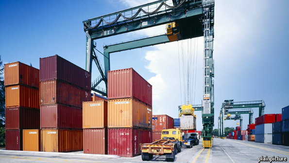
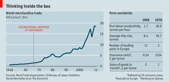
The effects of shipping container standardization is similar to the benefits of networking protocol standardization [Econ2013]. See Figure 2.

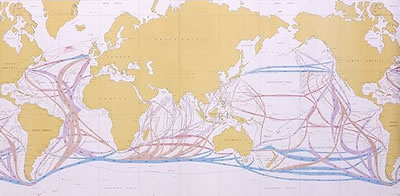
The trade routes used by shipping companies as shown in Figure 3 represent optimized path not unlike those used in packet or circuit switching.

Origins of Routing Protocols

The founders of the internet didn’t invent the concept of “routing”!  Shortest path algorithms such as Bellman-Ford (1956)  — used in RIPv2 — and Dijkstra’s algorithm (1959) — used in OSPF — came well before the internet! Note that T-carrier didn’t start to be deployed until 1962. These algorithms arose out of logistic/transportation problems similar to the package/container shipping examples we previously discussed.

Queueing theory, which we will be studying this semester, goes back to Markov (1906) and Erlang (1906 etc...). But we can still use this theory over 100 years later to tell us about the packet delays in an IP router, or the dropping (on handoff) of a cellular phone call.

So has everything been done before? Not really... Both the networking problem space and the technology available to address these problems keep changing.

Understanding a continuously changing field

Technology in general and networking in particular is continuously changing. This can make it very challenging to keep up with a field. However, the same or similar concepts tend to be revisited again and again in different technological guises.

As an example below is a list of historical and modern connection oriented packet networking technologies of which we will be studying MPLS this semester.

1. X.25 (1970s-today)  Formed the first national and international public data networks, well before the internet, well before the “OSI layer model”. Introduced the notion of “virtual circuit”. Variable sized packets.

2. Frame Relay (1988). Concepts included: “virtual circuits”, “committed information rate”, etc... Related to ISDN telephone standards... Variable sized packets.

3. Asynchronous Transfer Mode (ATM) (1994). Added concepts of virtual paths that could contain virtual circuits. Extensive control plane based on distributed routing and signaling. Fixed sized packets.

4. MPLS (2000). Variable sized packets. Allows arbitrary depth of label switched path (LSP) nesting. Distributed control plane leveraging IP routing protocols and including multiple "signaling like protocols" for label distribution.

Multiplexing and Inverse Multiplexing Concepts

The concept of multiplexing in wide variety of forms plays a key role in networking. Less well known but still very important is the concept of inverse multiplexing. We'll review both in general here.

Multiplexing

A general definition of multiplexing: The combining of multiple distinct entities into a larger containing entity for transport.

A general definition of demultiplexing: The extraction of distinct entities from a larger containing entity upon arrival from transport.

General overarching concept: Economies of Scale

Limits: Practicalities of bigger "containers".

Important implementation consideration: Telling the component entities apart without having to look too deep.

Human Transportation examples: Car pools, busses, trains, airplanes.

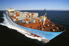
Package Transportation examples: multiplexing packages into trucks, airplanes, containers; containers into ships, and/or trains. Multiplexing in "container" switching is shown in Figure 4, i.e., how big is your boat.

Why bother with multiplexing in Networking?

The $N^2$ problem: suppose we have N entities that wish to communicate, how many communication channels do we need for this to take place?

Try drawing three node network and show how you would need need six unidirectional channels to allow all nodes to communicate with each other.  In general we need $N(N-1)$ unidirectional channels for $N$ communicating entities. The question is how to implement these channels.

What are the costs associated with a communications link?

1. Power

2. Bandwidth (frequency spectrum) – fundamental limit imposed by information theory for an additive white Gaussian noise channel $C_{awgn} = W log_2 \left(1+ \frac{P}{N_0W}\right)$

3. Receiver and Transmitter hardware costs (electrical, optical – lasers)

4. Transmission media: air (spectrum license), UTP, COAX, fiber

5. Media support: cable assembly, conduit, telephone poles, trenches...

If only the theoretical limits represented by (1) and (2) are present then how we implement the channels doesn’t matter all that much.  But items (3)-(5) are generally very important in real networks.

Can you afford a separate transmitter and reciever for every potential communication partner? Would you have space for them? ⇒ Pin count (or I/O) limitations.

Can you afford a separate wire or fiber optic cable between everyone you need to communicate with?

In reality the wires/fibers need to be within a protective cable assembly to withstand the elements, flora, and fauna. Trenches, telephone poles, and cable assemblies, along with their installation is frequently the most expensive aspect of a communication network.

Aside: General categories of expenses – (OpEx) Operational Expenses, (CapEx) Capital Expenses.  OpEx includes “Running costs” and CapEx includes “Installation costs”. There are frequently trade offs and optimizations between OpEx and CapEx in networking.

In general we will want to share expensive or scarce communication resources such as (a) receivers, (b) transmitters, (c) fiber, etc... amongst communicating entities.

Well look at two general types of communication modes bit streams and messages and their corresponding methods of resource sharing (multiplexing).

1. Time sharing

   1. for bit streams give each a repeating slice of time in a faster frame (TDM) T1 example 24 voice channels plus a framing bit.

   2. for messages give each a chunk of time on the channel (statistical multiplexing), Example Ethernet. But how do we tell messages or conversations apart?

2. Frequency sharing

   1. Allocation of radio frequency spectrum

   2. Allocation of optical spectrum in a fiber

3. Others

   1. Space division multiplexing

   2. Polarization mode multiplexing

   3. etc...

Multiplexing in packet switching:

• Statistical Multiplexing: Time slots — usually of variable length — are allocated for packet transmission but not reserved for a particular packet. This brings uncertainty about exactly when a packet gets transmitted that we'll look at when we study queueing theory. In the early days of packetized voice tranmission one of the simplest bandwidth saving techniques was to supress packet transmission if a user wasn't talking while this doesn't save bandwidth for a single voice channel it saved significant bandwidth when a number of voice channels are packetized this way and then combined. Such bandwidth savings were "statistical" in nature and hence the term statistical multiplexing.

• With packet multiplexing can't use only time slot or frequency to identify the packets of different users. Need some additional information to tell the packets apart. What is the minimal amount of information? (Some kind of label) What would be considered complete information? (a complete address of the destination) Think about link and network contexts.

• How do different networked applications running between the same two computers not get their packets confused? What facilities might be offered by the transport layer to help? What in particular do UDP and TCP offer for this? Where would this information be kept?

Inverse Multiplexing Concepts

What if the entity we wish to transport is too big for a single channel?

A general definition of inverse multiplexing is the coordinated use of multiple lower capacity channels to achieve a single higher capacity channel.

In a networking context this can be done on an end to end basis or a link basis. Like multiplexing, inverse multiplexing can be done at many layers.

Overarching concepts: Divide and conquer, Parallel Processing.

Limitations: Overhead increases as the number of "sub-channels" increases.

Implementation difficulties: reassembly of original "stream" in the presence of delays and errors.

Inverse multiplexing examples:

1. VCAT/LCAS is used with Layer 1 TDM technologies such as SONET, SDH, and G.709. End to end across a network. Specified in ITU-T G.707, G.7042, G.7043, G.709. For an overview see [VCAT2006]

2. MLPPP (multi-link point to point protocol) used in early days of the internet combined multiple low speed access lines (think dial-up or ISDN 64kbps channels).See RFC1990 [PPPMP].

3. Ethernet Link Aggregation Groups (LAG), IEEE Std 802.1AX-2014 [LinkAg].  This is a link level — not network end to end — form of inverse multiplexing. Why might you want or need this? Think about the sizes of Ethernet "pipes", e.g., 10Mbps, 100Mbps, 1Gbps, 10Gbps, 100Gbps. What if you needed something in between?

4. Equal Cost Multipath ECMP can be thought of as a form of inverse multiplexing at layer 3. See also RFC2992 [ECMP2000]. Note that this has similar limitations to Ethernet LAGs.

5. Multipath TCP [MTCP2011]; [MTCP2013]. This is an "experimental" protocol from the IETF. Implementations are available for Linux and some proxy clients.

6. Bit Torrent (Application layer)

Digression: Standards and Networking

Why are standards so important in networking compared to other high technology fields?

1. Networks will not operate without equipment compatibility at many levels

2. Distributed and global scope

3. Carriers, ISPs, and Enterprises are reluctant to get “locked-in” to a single vendor's solution..

Standards Development Organizations (SDOs) we will use frequently in this course:

1. IETF (Internet Engineering Task Force), They issue RFCs some of these are informational, some are “standards track”. Always freely available.

2. ITU-T (International Telecommunications Union, Telecommunications sector) issues “recommendations”.  Almost all are now freely available. We'll be looking at their documents for optical networking.

3. IEEE (Institute of Electronic and Electrical Engineers) Issues “standards”.  Only a small subset are freely available. We’ll use the series 802 documents.

4. Open Networking Forum (ONF) maintains and updates the OpenFlow software define networking (SDN) specifications and has many other projects and activities.

Layers and Partitions in Networks

You should have been exposed to the Open Systems Interconnection Model along with a similar flavored TCP/IP model in a previous networking course. If not the previous Wikipedia links provide more than enough information for a thorough review. As you continue your networking career you will encounter many examples of layered networking models adapted to the particular problem at hand.

In you previous networking class you may have learned about local area networks (LANs) and compared them to wide area networks (WANs). You may have seen that the size and extent of a network domain called for different data and control plane techniques. During this class we'll expand on both these of "vertical" and "horizontal" decomposition of networks.

Network Layering: beyond the OSI model

Why layers in networking?

• A way to separate network functionality for reuse
  • Put the smallest usable sub-set of functionality into a layer
  • Isolate dependencies behind a general purpose interface. Analogous to good software architecture.
• A way to incrementally add functionality
  • Not all communications need the same treatment with respect to reliability, QoS, etc...
  • Types of functionality: multiplexing, communications reliability, performance monitoring, inverse multiplexing, multi-casting, etc...
• A way to demarcate interoperability interfaces
  • Software and Hardware!
  • Packets, bit streams, electrical, and optical

Examples:

The seven layer OSI model from Wikipedia:

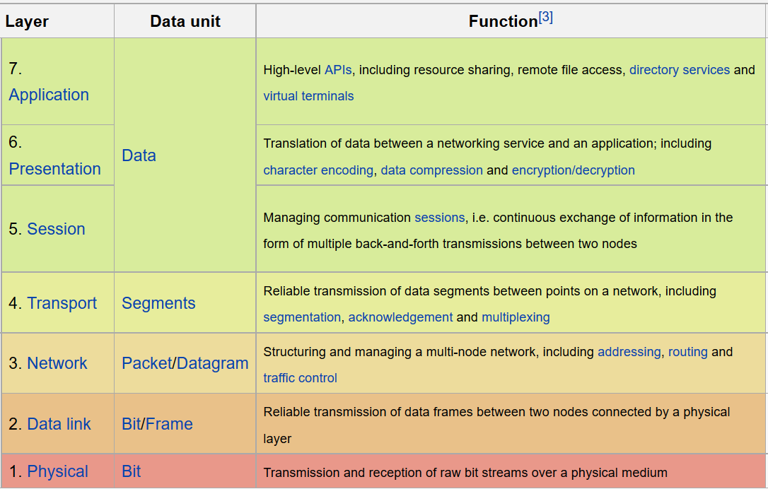
Internet Layer Model:

A protocol specific stack example:

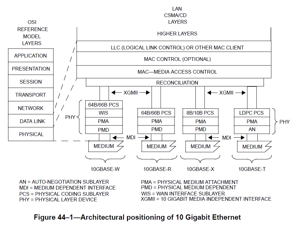
10 Gigabit Ethernet Layer Model:

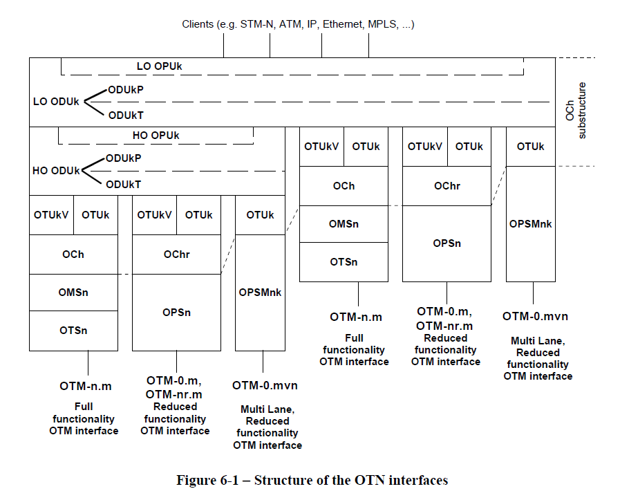
Optical Transport Network (OTN) layer model:[ITU-T2012]

Don't worry if you don't understand any of this now.

Multi-Path TCP stack — they split the transport layer! —:

                                   +-------------------------------+
                                   |           Application         |
      +---------------+            +-------------------------------+
      |  Application  |            |             MPTCP             |
      +---------------+            + - - - - - - - + - - - - - - - +
      |      TCP      |            | Subflow (TCP) | Subflow (TCP) |
      +---------------+            +-------------------------------+
      |      IP       |            |       IP      |      IP       |
      +---------------+            +-------------------------------+

      Figure 1: Comparison of Standard TCP and MPTCP Protocol Stacks

Explanation of the split from Multipath TCP architecture document.

          +------------------+
          |    Application   |
          +------------------+  ^ Application-oriented transport
          |                  |  | functions (Semantic Layer)
          + - - Transport - -+ ----------------------------------
          |                  |  | Network-oriented transport
          +------------------+  v functions (Flow+Endpoint Layer)
          |      Network     |
          +------------------+
            Existing Layers             Tng Decomposition

              Figure 4: Decomposition of Transport Functions

Network Partitions

Besides layering how else do we "divide and conquer" our networks? In addition to layers we also partition networks amongst subsets of network elements including links. Typical general term applied to this process are “domains”, "sub-domains", "sub-networks".

Example network partitions:

• Link — just two nodes and the link connecting them —
• Local Area Network (LAN). Historically and even today the "domain" where broadcast protocols are used. An example of an extremely important broadcast protocol is the address resolution protocol (ARP).
• Metropolitan Area Networks (MAN). Usually run by a single internet service provider (ISP) or carrier. Scope is a single small to large metropolitan area.
• Wide Area Network (WAN).
• OSPF routing area. A control plane defined "sub-network" of the OSPF routing protocol.
• BGP Autonomous systems. The border gateway protocol (BGP) works between "sub-networks" called autonomous systems (AS). An AS can contain many

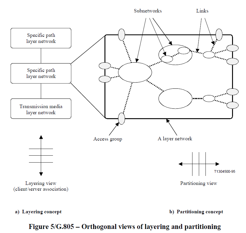
Layers and partitions give us two different ways to view and decompose networks. From ITU-T G.804:

Data and Control Planes

Every switching like device must have rules or procedures for directing inputs to various outputs. In many cases these rules or procedures have parameters or will take instructions that control the switching process. We'll call these rules or procedures the data plane of a switch since they are directly involved with switching the inputs to the outputs.

What makes things somewhat confusing is that the data plane may be implemented in hardware, software, or a combination of the two depending on the technology. Think about the different implementations used for an optical switch, a large carrier router, a wireless home router, or a virtual switch used between virtual machines running on the same processor.

We'll call the techniques we use to set the parameters or instructions that we can give to the forwarding rules or procedures the control plane since the configuration of these will control the behavior of the switch. We'll see lots of different control plane examples for different switching types from wavelength switched optical network elements to virtual switches that implement the OpenFlow protocol. Almost all switches have at least a rudimentary control interface. When we put multiple devices into a network we have more interesting examples of control planes that will coordinate the setting of the device parameters to achieve a (hopefully) functioning network.

Switches, Ports, and the Forwarding Table

Once we move beyond single links connecting two entities, we will be dealing with network elements that we will generically refer to as switches. More specific terminology may be used when we talk about a particular technologies, i.e., IP routers, label switched routers (LSRs in MPLS), reconfigurable optical add/drop multiplexers (ROADMs in optical networking), Ethernet bridges, etc..., however this terminology sometimes obscures rather than illuminates so we will frequently just use the term switch and indicate what layer we might be using. Still more confusing, many switches can work at multiple layers (particularly SDN devices), hence we'll call them all switches.

Switches have input and output ports from which they receive and send the information that they are forwarding. The links that connect to the switch ports may use a variety of multiplexing schemes and a switch may be able to demultiplex one or more of these schemes, i.e., discriminate on, and this is roughly what we mean by the layer of the switch. For example IP router with Ethernet interfaces would be forwarding at the IP layer and not the Ethernet layer. An Ethernet bridge on the other hand bridge doesn't look at the IP layer information.

Conceptually every switch can be thought of as having a forwarding table. At its simplest this could be direct all the inputs on a given port to be output on another port. In more complicated cases it may contain specific selection criteria for packets and instructions for selective copying and forwarding of the packet.

Example switch/multiplexing schemes:

• TDM – time slots
• WDM – wavelengths (frequency)
• Ethernet Switches
• IP router
• SDN switches

All switches conceptually have some type of table that maps (ingress port, incomming multiplexing id) to (egress port, possibly new outgoing multiplexing id)

Example 1.  Old fashioned DS1 cross connect.

Example 2. WDM wavelength selective switch

Example 3. Ethernet switch (more complicated rules, but still has the notion of a forwarding table, though this concept is not in the IEEE standard).

Beyond the Control Plane: The Management Plane

In addition to the data and control planes which we will cover, there are a number of critical functions for running a network that we will not be covering in this class these include:

• fault detection, isolation, and recovery
• performance monitoring and capacity planning
• network security in general
• general network configuration

Some of these fall under the category of network management, and others are vast topics in their own right.

As an aside, a traditional way to remember management plane functions was via the accronym FCAPS:

• Fault – Detection (has something gone wrong), Isolation (where exactly is the problem), Recovery/Mitigation

• Configuration – installation, equipment setup, maintenance of forwarding tables, etc...

• Accounting – who is using how much of a resource and when

• Performance – BER, delay, delay variation, etc...

• Security

Control versus Management Plane:

Control planes tend to be distributed and focused primarily on a small subset of configuration and fault recovery.  Examples include OSPF, BGP, RSVP, etc...

Review: Ethernet Switching (Bridging)

Throughout this course we will utilize examples based on Ethernet technology and refer to Ethernet standards documents. One of the main things that makes Ethernet specifications hard read is that the terminology utilized stems from a fairly long and distinguished history starting with the first commercialization of Ethernet in 1980. Wikipedia has good overview of Ethernet and its history.

The first thing to remember is that Ethernet started life as as shared medium technology (Thicknet, Thinnet, and Hubs). Low port count bridges were then used to interconnect segments of shared medium. Since Ethernet started life as a shared medium technology where all packets were broadcast it was natural to use the term filtering with an Ethernet bridges to specifying which packets were forwarded between two LAN segments, i.e., the default was broadcast. However, for those of us who mostly think in terms of point to point (rather than shared medium broadcast) cabability for wired networks the term filtering in a switching device brings up notions of firewalls and such. This is not what is intended by the term filtering in the IEEE 802.1D (bridging) specification.

Ethernet history from the switching point of view:

1. Thicknet (shared medium, fat coaxial cable with taps for each host) CSMA-CD

2. Thinnet (shared medium, thinner coaxial cable with BNC connectors for easier connection to hosts) CSMA-CD

3. Hubs and UTP (unshielded twisted pair to hub, still acts as a shared medium) CSMA-CD

4. Low port count “Bridges” to interconnect shared medium LANs. ==> Small switches.

5. High port count bridges ==> completely switched Ethernet networks. Essentially no more CSMA-CD.

6. Feature rich Ethernet switches including VLANs and more. Precursor to Software Defined Networks (SDNs).

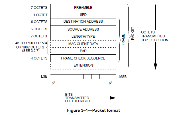
The progress in the switching capabilities of Ethernet over time has been over shadowed by the progress of Ethernet as link technology. The current IEEE 802.3 (2012) specification for the Ethernet link — medium access control (MAC) — technology is divided into six sections consisting of 90 chapters (clauses) and covers link speeds ranging from 10Mbps to 100Gbps — that's five orders of magnitude!. We'll look at the highest speeds of Ethernet when we study optical networking. Fortunately for all the different speeds the basic Ethernet frame structure has remained the same!

Ethernet Switching

Ethernet switching (Ethernet Bridging) is defined in the IEEE 802.1D-2004 standard. As mentioned before the terminology utilized in the standard may make it a little bit harder to see our data, control, and management plane model of networking but they are in there!

1. Forwarding behavior is dictated by a "forwarding" table (though its not called that)
2. The switching network topology is restricted to a tree (if it contains loops) by the use of a distributed control plane protocol running between switches. Not all switches have this capability.
3. The "forwarding table" is filled in by a control plane process called the learning process. This isn't coordinated between switches (hence the need for the previous step).
4. More feature rich switches will have some type of management interface for access to the management plane functionality (FCAPS).

Populating the Ethernet Forwarding Table

The hidden "Ethernet control plane" is the learning process from the IEEE 802.1D-2012 standard. Without covering all the corner cases or using the proper standards language we will summarize the procedures here. First of all we are assuming that the network has a tree topology. This implies that there is only one path between any two nodes (hosts) in the network. What the Ethernet switches need for their forwarding table is to know on which port to forward an Ethernet frame bound for a particular Ethernet destination address. The algorithm works at follows (we cover only the unicast case here):

• Upon reception of a frame a switch will:
  1. Record the input port # and the source address of the packet.
  2. Since the network has a tree topology there is only one path that this frame could have used to reach this switch and if we ever need to send a frame to the source address from above we should use the output port corresponding to input port we saw above.
  3. If an entry with (Ethernet address, port) corresponding to the above is not present in the forwarding table add it, otherwise reset the ageing time for the table entry.
• To forward a received frame:
  1. If there is no entry in the forwarding table that matches the destination Ethernet address, forward the packet out all (active) switch ports except the port on which the packet was received. This step alone would emulate an Ethernet hub with a switch. This is also the step that results in disaster if the network topology is not a tree!
  2. If there is an entry in the forwarding table only forward the frame out that particular port.
• Periodically: Check the forwarding table entries and remove those that have expired.

Pretty cool and simple! We'll see this algorithm again when we look at SDNs since it is about the simplest non-trivial control plane one can implement via an OpenFlow controller and is featured in many SDN tutorials.

References

• [Econ2013]  “Why Have Containers Boosted Trade so Much?”, The Economist, May 2013.
• [VCAT2006]  G. Bernstein, D. Caviglia, R. Rabbat, en Huub van Helvoort, “Standards: VCAT/LCAS in a Clamshell”, IEEE Communications Magazine, vol 44, no 5, 2006.
• [PPPMP]  T. Coradetti, K. Sklower, D. Carr, G. McGregor, en B. Lloyd, “The PPP Multilink Protocol (MP)”, Aug-1996. Available at: https://tools.ietf.org/html/rfc1990.
• [LinkAg]  “IEEE Standard for Local and Metropolitan Area Networks – Link Aggregation”, IEEE Std 802. 1AX-2014 (Revision of IEEE Std 802. 1AX-2008), bll 1–344, Des 2014.
• [ECMP2000]  C. E. Hopps, “Analysis of an Equal-Cost Multi-Path Algorithm”, 2000. Available at: https://tools.ietf.org/html/rfc2992.
• [MTCP2011]  M. Handley, C. Raiciu, A. Ford, J. Iyengar, en S. Barre, “Architectural Guidelines for Multipath TCP Development”, Mrt-2011. Available at: https://tools.ietf.org/html/rfc6182.
• [MTCP2013]  M. Handley, O. Bonaventure, C. Raiciu, en A. Ford, “TCP Extensions for Multipath Operation with Multiple Addresses”, Jan-2013. Available at: https://tools.ietf.org/html/rfc6824.
• [ITU-T2012]  ITU-T, “Interfaces for the Optical Transport Network”, Feb 2012.