Introduction

In this section of the course we give a brief but wide introduction to optical networking. Unlike other portions of the course where most of us have had some hands on experience with the technology, high speed optical networks while forming the backbone of the Internet and most private high speed networks remain hidden from view in data centers, carrier central offices, in submarine cables spanning oceans, buried in trenches, etc. We'll emphasize here what makes optical networks so special, key optical components, optical multiplexing, and special considerations needed for the optical control plane.

Optical Networking History

One could argue that optical networking pre-dated electronic forms of communications, i.e., Armies in ancient times used signal flags for sending messages. However, here we are interested in communications over optical fiber. At first glance it may seem like shining a light down a glass fiber for communications purposes is not such a revolutionary concept. But that is not the case! At least three of the technologies/ideas that are common in optical networks today earned their inventors/discoverers Nobel prizes in Physics:

1. 2009 Nobel Prize in Physics C. K. Kao for “for groundbreaking achievements concerning the transmission of light in fibers for optical communication”. See http://www.nobelprize.org/nobel_prizes/physics/laureates/2009/popular-physicsprize2009.pdf. We'll look at the key properties that make optical fibers so special in the next section.

2. 1964 Nobel Prize in Physics for the “invention of the Laser” (C.H. Townes, N.G. Basov, and A.M. Prokhorov). Lasers of all different types are used as the transmitters (sources) in optical networks.

3. 1930 Nobel Prize in Physics. C. Venkata Raman “scattering of light”. Though we will not go into detail here. You will see the name "Raman" associated with an important type of optical amplifier when we discuss optical components.

Modern Timeline:

Kao’s work published 1966, Corning made first experimental fiber 1970, First production (non-experimental) link 1975, First transatlantic optical cable installed in 1988. Erbium-doped fiber amplifiers 1989, Commercial DWDM systems ~1996. Very good modern technical history can be found in the “preface” of the ITU-T Handbook.

Optical Fiber

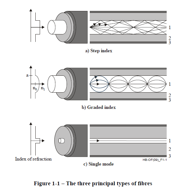
The two fundamental properties of modern optical fiber that make them so attractive for communications use are their: attenuation and bandwidth. Due to various technical and economic considerations there are two main types of fiber in common use multi-mode fiber (MMF) and single-mode fiber (SMF). With MMF the fiber core is large compared with the wavelength of the light used and we can imagine the light rays reflecting off the inside of the fiber as they propagate. With SMF this isn't the case and a more complete analysis based on Maxwell's equations are needed to understand the propagation.

1. Multimode fiber –

   1. core diameter 50μm

   2. cladding 125μm

   3. typical transmission wavelength 850nm, lower cost transmitters available. Commonly used for 10Gbps Ethernet in data centers.

   4. Propagation via total internal reflection.

2. Single Mode fiber –

   1. core diameter 8-10μm. Makes this fiber harder to work with and various parts more expensive.

   2. cladding 125μm

   3. typical transmission wavelength 1300-1550nm

   4. Internal reflection picture not accurate, need to use Maxwell’s equations.

Attenuation

All electro-magnetic communication signals degrade when transported over some type of physical medium (electrical wires, fiber optic cable, free space). One of the most important degradations is attenuation which is the reduction in signal amplitude/power caused by losses in the transport medium. In optical communications we tend to work with signal power rather than amplitude. In addition because we can tolerate a very wide range of losses we use a logarithmic scale to quantify those losses, in particular we use the units of decibel (dB).

The decibel is defined as a logarithmic ratio of output to input power:

$$dB = 10 \log_{10}\frac{P_{out}}{P_{in}}$$

Example: Suppose that $P_{in} = 1mW$ (that is one mili Watt) and that $P_{out} = 1\mu W$ (one micro Watt) then the attenuation in dBs is: $10 log_{10} (10^{-3}) = -30dBs$.

We can get back our output power from the input power and dB loss (or gain) by simply taking the exponential:

$$P_{out} = P_{in} \cdot10^{\frac{dB}{10}}$$

We also use decibels to talk about optical amplifier gain and to talk about signal power relative to a 1mW standard. We have

$$dBm = 10 \log_{10}\frac{P}{\mathrm{1mW}}$$

Example: What is the power in dBm of a 2mW laser transmitter? Answer: $10 \log_{10}(2) \approx 3.01 dBm$.

Given the loss in dBs we can define the attenuation in terms of the loss in dBs over distance.

$$\alpha = \frac{10}{L} \log_{10}\frac{P(0)}{P(L)}$$

Notice that the ratio inside the log is "flipped" so that attenuation is always positive, i.e., a bigger number means more loss per distance.

One of the problems with electric cables of all types (UTP, Coax, etc.) is that the attenuation gets worse with higher frequency (bandwidth) signals. For modern (electrical) coaxial cables operating near 10Ghz the attenuation is approximately 0.25dB/foot. However, for modern SMF fiber optic cables operating near 1550nm attenuation is approximately 0.2dB/km. Yes, that is per foot versus per km!!! Over three orders of magnitude of improvement with modern optical fiber! Note attenuation per kilometer for MMF at 850nm ~ 2.5 dB about 10 times worse than SMF.

For a more concrete example let's look at the maximum distances specified for 100Gbps Ethernet from IEEE 802.3-2012 Section 6, Chapter 80 Physical layers:

1. 100GBASE-CR10 at least 7 m over a copper cable assembly

   100 Gb/s PHY using 100GBASE-R encoding over ten lanes of shielded balanced copper cabling

2. 100GBASE-SR10 at least 100 m on OM3 multimode fiber (MMF)

   100 Gb/s PHY using 100GBASE-R encoding over ten lanes of multimode fiber,

3. 100GBASE-LR4 at least 10km on single-mode fiber (SMF)

   100 Gb/s PHY using 100GBASE-R encoding over four WDM lanes on single-mode fiber

4. 100GBASE-ER4 at least 40km on single-mode fiber (SMF)

   100 Gb/s PHY using 100GBASE-R encoding over four WDM lanes on single-mode fiber

Bandwidth

The attenuation with wavelength for typical SMF optical fiber is shown in Figure 2.

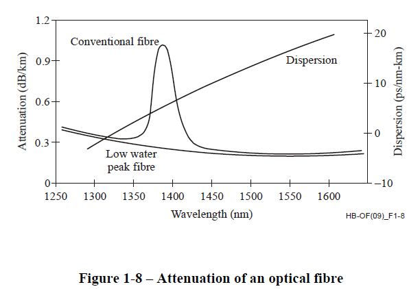
Due to the large rise in attenuation for conventional due to water absorption and historical developments it has been common to break the range of potential useable wavelengths into named spectral bands as shown in Figure 3

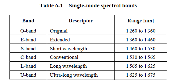
Let's look at an example of the bandwidth (in frequency) of the C-band. To convert from wavelength to frequency we just use the fundamental relation: $f = c/ \lambda$ where $c = 299792458 m/s$ the speed of light. For the short end of the C-band we have $c/1530x10^{-9} = 195.9428THz$ and for the long end of the C-band we have $c/1565x10^{-9} = 191.5607THz$ (note that THz = $10^{12}Hz$). To get the total bandwidth in the C-band we subtract these to get approximately $4.38THz$ of raw bandwidth! For comparison the entire conventional radio spectrum fits within a range of 30GHz over two orders of magnitudes smaller and that is just one optical band!

One more thing we should mention is that since optical fibers have such small diameters and need to be protected when carriers lay cable the "cable" actually contains a bundle of fibers.

Multiplexing over Optical Fiber

Although optical fiber has imense bandwidth , digital electronics cannot currently run at clock rates near that of fiber bandwidth, hence we need a way to utilize the bandwidth potential based on lower rate digital channel. In analogy with frequency division multiplexing of the radio spectrum we can give different "lower rate" digital channel a separate wavelength/frequency of light on the same fiber as long those channels do not interfere with each other. In optical communications this is known as wavelength division multiplexing (WDM).

There are two standards covering wavelengths and channel spacing. ITU-T Recommendation G.694.1, "Spectral grids for WDM applications: DWDM frequency grid" [G.694.1], describes a dense wavelength division multiplexing (DWDM) grid defined in terms of frequency grids of 12.5 GHz, 25 GHz, 50 GHz, 100 GHz, and other multiples of 100 GHz around a 193.1 THz center frequency. At the narrowest channel spacing, this provides less than 4800 channels across the O through U bands. ITU-T Recommendation G.694.2, "Spectral grids for WDM applications: CWDM wavelength grid" [G.694.2], describes a coarse wavelength division multiplexing (CWDM) grid defined in terms of wavelength increments of 20 nm running from 1271 nm to 1611 nm for 18 or so channels.

ITU-T recommendations can be downloaded for free from http://www.itu.int/itu-t/recommendations/index.aspx?ser=G.

Basic Optical Systems

Digital Optical Signals

The first widely deployed standard high capacity signals were the SONET/SDH signal hierarchies. In Figure 4 we show an example TDM frame. Each small block represents a byte and the entire frame is repeated every 125uS. SONET and SDH are essentially the same with somewhat different terminology. The unusual frame size for the basic SONET/SDH signal shown below was partially due to the need to carrier both North American (T1) and Europen (E1) digital voice signal hierarchies. The signal rates for the SONET/SDH multiplexes (rather than the tributary, i.e., component signals) range from 155Mbps, to 40Gbps. The "synchronous payload evelope" is the area that contains the user byte stream (this isn't a packet). The various named bytes such as "A1" or "J0" serve important functions such as performance monitoring, fault isolation, protection switch, etc... We will give concrete examples for the case of the G.709 digital signal hierarchy to be discussed later.

To go beyond standard Ethernet electrical cabling distances, optical interfaces and fiber were introduced into the IEEE 802.3 series of specifications. Hence the familiar Ethernet frame is another example of a digital signal frequently used over optical interfaces.

Finally we have the G.709 TDM signal hierarchy that is typically used in high rate WAN (metro, long haul, ultra-long haul) systems. As Show in Figure 5 this is a quite elaborate signal. So why bother with a TDM frame structure when most of the traffic carried is packets?

• The efficiency of TDM switching at a given rate compared to packet switching. Hence for very high data rates TDM switching has advantages.
• The ease of providing rigorous QoS guarantees with TDM, rigid "walls" prevent DoS style attacks.
• The need for FEC over the same size blocks
• Low overhead but very responsive fault alerting, localization, and performance monitoring.

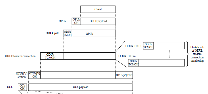
However essentially a client signal is put into an optical channel payload unit (OPUk) which is then put into an optical channel data unit (ODUk) which is then place into an optical channel transport unit (OTUk). The general purpose of each of these layers is:

• OTUk: this is the actual digital signal that gets encoded and modulated onto a particular wavelength. This signal exists between a single channel optical transmitter and a optical-electrical-optical regenerator or receiver. This is the signal that has forward error correction (FEC) coding added to reduce the bit error rate on WAN links. These currently come in four flavors OTU1 through OTU4 with bit rates of approximately 2.5Gbps, 10Gbps, 40Gbps, and 100Gbps.

• ODUk: The main purpose of this layer is to provide what is called tandem connection monitoring. Client signals are typically assured of a maximum end-to-end bit error rate. When a user signal is passed between multiple networks or subnetworks it is important to know how much each subnetwork/network contributed to the overall bit error rate. The ODUk provides for error monitoring for six sets of "network demarcation points". --> Also protection switching see G.808.1-.3 series, communication channels... The smallest capacity is an ODU0 with a rate of approximately 1.25Gbps. There are many more types of ODU signals than OTUk signals as these along with the OPU signals are also used to adapt 10Gbps, 40Gbps and 100Gbps Ethernet into OTUk signals for WAN transport.

• OPUk: Provides adaptation of the client signal and/or multiplexing of client signals. When used to multiplex client signals these "containers" can support signals of either 1.25Gbps or 2.5Gbps. There are many standardized and proprietary methods for mapping (adapting) various digital signal (including packet streams) into OPUs.

To get a flavor of how G.709 works the structure of the OTUk signal is shown in Figure 6 . The signal uses a row/column byte structure of 4 rows with the first 15 columns devoted to overhead for the OTUk, ODUk, and OPUk signals and the last 256 columns are used for forward error correction (FEC). Not counting the FEC we can compute the efficiency of the OTUk signal as 99.6% or an overhead of only 0.4%. This is extremely small even though there is a great deal of important functionality in the overhead. To create the faster OTUk signals the repetition period for the signal is shortened. For example for an OTU1 the period is 48.971uS while for an OTU4 the period is 1.168uS (see table 7-5 of G.709).

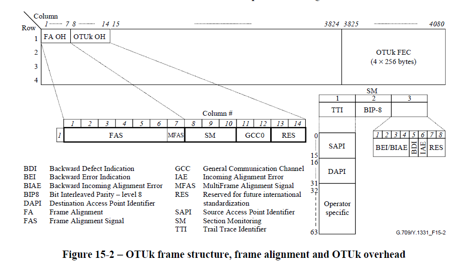
Let's take a quick look at what some of the overhead bytes are for and why they are so useful.

• Frame Alignment overhead The frame alignment signal (FAS) is just a fixed set of six bytes that identifies the start of the frame. It is by recognizing and aligning with these bytes that we can get at all the other overhead bytes and the payload. we do not need to realign with each frame, in general the frame alignment procedure will take many frames to complete and the link is not declared operational until frame alignment has been acheived. The multi-frame alignment signal (MFAS) allows us to identify a repeating sequence of 64 frames to form a "multi frame". This allows us to divide a single overhead byte into 64 bytes (one for each frame in a multi frame). This is used in section monitoring.

• General Communications Channel 0 An OTUk may be the only communication signal between to points. Since we are dealing with time slots rather than packets we cannot insert management or control packets into the payload, instead the OTUk provides two bytes of overhead for general (management or control) communications. At an OTU4 rate this would provide a 13.6Mbps dedicated channel completely isolated from user traffic (sometimes called an out of band channel).

• Section Monitoring (OTUk) provides bit error estimation, end point identification, and a variety of alarm signals. See G.709 section 15.7 for complete details.

  • The BIP-8 byte in the SM section contains a parity check code over all the bytes in the payload and some of the header of a frame as computed by the OTUk source, the same computation is performed at the receiver and comparing the two gives a bit error count for the frame. This works extremely well since the FEC corrected error rate of an optical link is quite low. We essentially get real time updates of the line bit error rate from the BIP-8!

  • How do we know if how well the receiver is hearing our signal? The byte after the BIP-8 contains bit or multi-bit signals to let us know. These have names such as Backward Error Indication (BEI) and Backward Defect Indication (BDI) that the receiver uses to tell the source about the bit errors its received and whether the link is considered defective.

  • How do we know the source and intended receiver for the signal? The Trail Trace Identifier (TTI) serves this purpose. You get 16 bytes for source identification and 16 bytes for destination identification. Typically simple ASCII character strings are used. We'll see the use of these bytes in GMPLS "discovery" process.

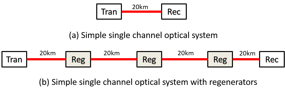
Single Channel Systems

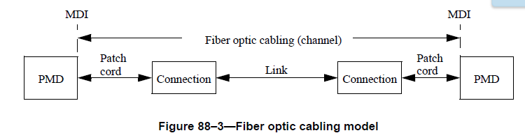
The simplest optical systems consist of a transmitter, optical fiber, and a receiver. Such systems are used in data centers and other moderate bandwidth, relatively short distance environments (note that these distances can be quite long compared to electrical cabling!).

For longer distances we need to regenerate the signal before it degrades (due to attenuation, noise, and other propagation effects) so much that the bit error rate gets too high to allow for reliable communications. There are a number of ways we can regenerate the signal: re-amplify it, reshape-it, or re-time it. The formal definition of these three types of regeneration (1R, 2R, and 3R) is given in the table below from ITU-T G.872/IETF RFC6163:

   --------------------------------------------------------------------
   1R | Equal amplification of all frequencies within the amplification
      | bandwidth.  There is no restriction upon information formats.
      +----------------------------------------------------------------
      | Amplification with different gain for frequencies within the
      | amplification bandwidth.  This could be applied to both single-
      | channel and multi-channel systems.
      +----------------------------------------------------------------
      | Dispersion compensation (phase distortion).  This analogue
      | process can be applied in either single-channel or multi-
      | channel systems.
   --------------------------------------------------------------------
   2R | Any or all 1R functions.  Noise suppression.
      +----------------------------------------------------------------
      | Digital reshaping (Schmitt Trigger function) with no clock
      | recovery.  This is applicable to individual channels and can be
      | used for different bitrates but is not transparent to line
      | coding (modulation).
   --------------------------------------------------------------------
   3R | Any or all 1R and 2R functions.  Complete regeneration of the
      | pulse shape including clock recovery and retiming within
      | required jitter limits.
   --------------------------------------------------------------------

In Figure 7 we show a single channel system with and without 3R regeneration.

Wavelength Division Multiplexing Systems

In Figure 8 we show a representative drawing of a simple CWDM (coarse wavelength division multiplex system) such as those used for 100G Ethernet.

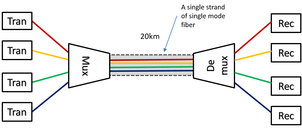
Optical demultiplexers for 100G ethernet IEEE standards presentation.

• Example WDM Link: 100GBASE-LR4

“The maximum link distances for single-mode fiber are calculated based on an allocation of 2 dB total connection and splice loss. For example, this allocation supports four connections with an average insertion loss per connection of 0.5 dB.”

Link details and power budgeting:

1. Frequencies/Wavelengths used: 231.4, 230.6, 229.8, 229.0 THz (1295, 1300,1304, 1309nm)

2. Average Transmitter power (minimum) per wavelength -4.3dBm (0.37mW)

3. Necessary Receive power (minimum) per wavelength -10.6dBm (0.087mW)

4. Cable attenuation max 0.43dB/km

5. Maximum cable length 10km

6. Worst case loss (attenuation) per connection 0.5dB

Do the math: -4.3dBm (xmit power) -0.43dB/km x (10km cable) – 4 (connections) x (0.5dB) = -10.6dBm  ==> necessary receive power!

Longer Haul DWDM Optical systems

For longer haul high capacity systems many more wavelength are used, typically in the range of 20-100. This requires more frequency stable laser transmitters as the spacing between the separate channels goes down. Hence the cost of the transmitters for long haul systems is greater than other system types.

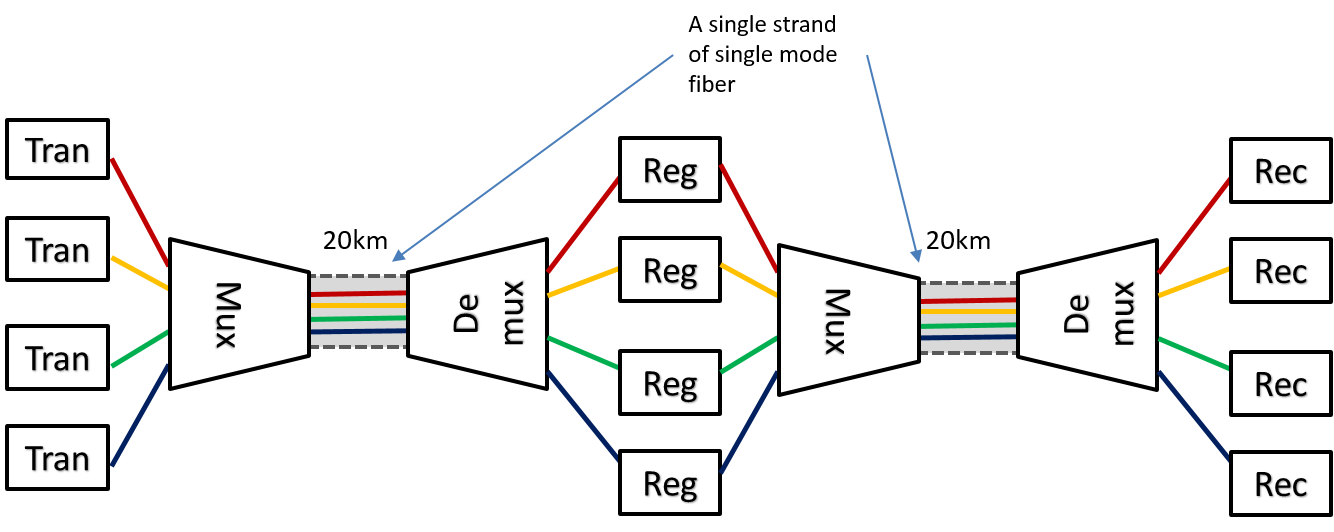
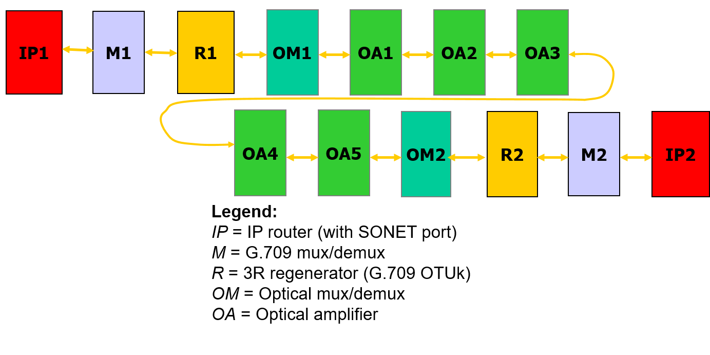
If we go longer distances it seems we would need to use regenerators as shown in Figure 11. We see from this picture that a very large number of regenerators are required (and these also need expensive laser transmitters).

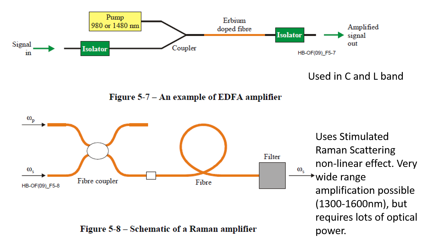
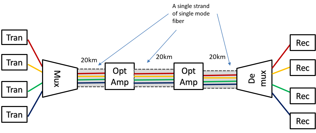
In the mid to late 1990s a breakthrough was made with the invention of the (all) optical amplifier. This device has the ability to amplify multiple channels of a DWDM signal (multiple light wavelengths) at the same time without intermediate conversion to an electrical signal. Block diagrams of two types of implementations are shown in Figure 12. This leads to much more cost effective long haul systems as shown in Figure 13 .

Terminology note You may see the abbreviations UHC (ultra high capacity) and UHL (ultra long haul) used to designate long haul DWDM systems optimized for high channel count and maximum distance between regeneration points, respectively.

Optical Networks

There are three forms of switching commonly used within optical networks:

• "True" optical switching of either an entire WDM signal or selective switching based on individual or ranges of optical wavelengths.

• Time division multiplex (TDM) switching: This requires optical to electrical conversion, switching takes place in the electrical domain, then reconversion from electrical to optical signals.

• Packet switching: This requires optical to electrical conversion, electrical packet switching, then reconversion from electrical to optical signals.

Key properties of these different switching types:

• Granularity (smallest amount of bandwdith that can be switched): Optical switching works at the coarsest level of granularity at its finest it can work with individual wavelengths that generally carry 10Gbps-40Gbps signals. High speed TDM signals typically can be switched in 1Gbps increments but some types have component signals of 50Mbps or less. Finally packet switching offers the finest granularity switching since an individual packet can be switched between any pairof destinations.

• Energy/Cost (per bit switched): Optical switching is the most energy efficient form of switching, followed by TDM switching, with packet switching being the most energy consuming.

Due the differing nature of these switching types a modern high capacity full service network will contain more than one switching type.

A Key Missing Piece While optical technologies have improved immensely in the last four decades one important component still does not exist: an all optical wavelength converter, i.e., a device that can efficiently convert from one optical wavelength to another while remaining in the optical domain. Currently all practical wavelength converters are optical-electronic-optical systems like a 3R regenerator. The wavelength conversion aspect comes from using a tunable laser transmitter. Hence wavelength conversion is as expensive as 3R regeneration.

We generally classify optical networks into three types:

• Transparent All switching is done optically and no wavelength conversion or regeneration takes place within the network, but only at the network edge.

• Translucent Uses a combination of optical and electronic switching, and may contain wavelength convertion or regeneration.

• Opaque All switching is done electronically. Optical technology including WDM is only used on the links. Optical to electrical conversion is done at every switch.

Optical Switches

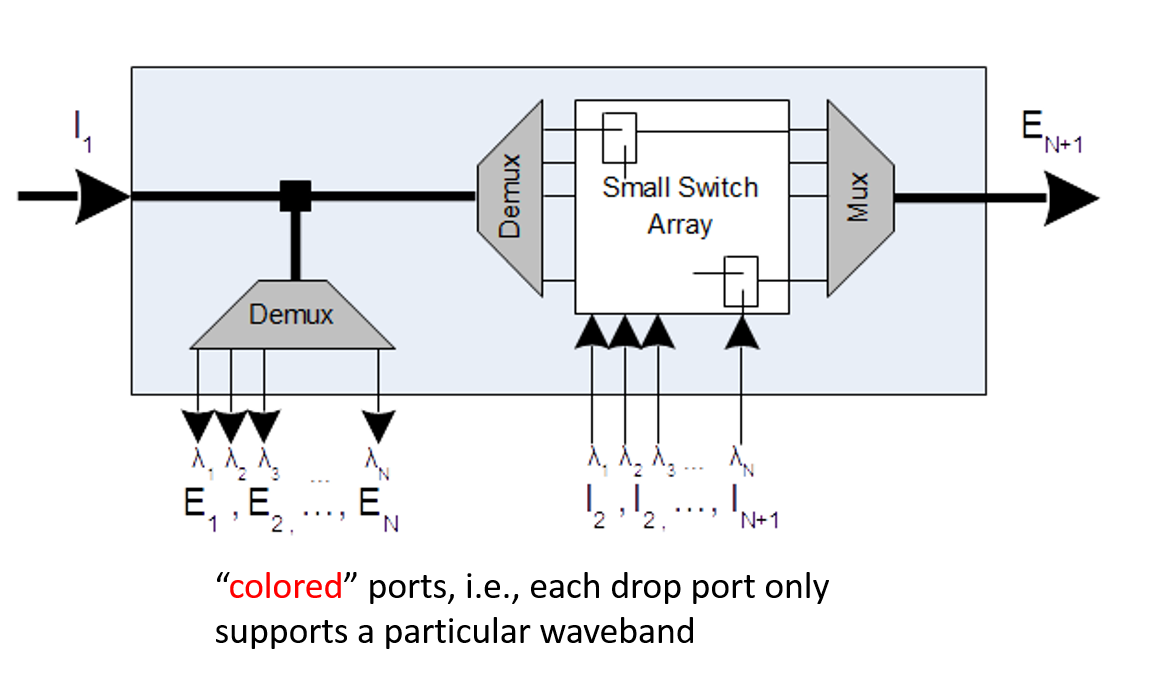
Optical switching like all other optical technologies has continued to advance. Here we will look at the a couple early designs of a very important optical switch known as a Reconfigurable Optical Add/Drop Multiplexer (ROADM). These are typically used in optical transport systems at intermediate points to "drop" off and "add" signals. In Figure 14 we show a block diagram of an implementation of a type 1 ROADM. The input port $I_1$ takes in a multi-wavelength WDM signal while the input ports $I_2,..., I_{N+1}$ take in single wavelength of a specific frequency. Similarly the output (egress) ports $E_1,...,E_N$ work with a single specific wavelength, while $E_{N+1}$ carries a WDM signal. In addition to these restrictions the WDM signal flow through this device is from left to right so none of the input signals from ports $I_2,..., I_{N+1}$ can be switched to ports $E_1,...,E_N$. This is very different from what we are used to with TDM and packet switches that do not have these types of port-to-port reachability constraints.

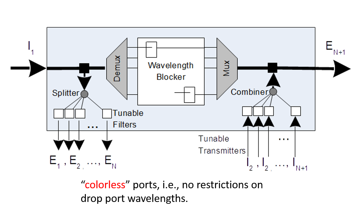
In Figure 15 we show a next generation of ROADM (type II). This features a wavelength blocker rather than a small switch array. The notable advantages over the type I ROADM are that the egress ports $E_1,...,E_N$ and not dedicated to a specific wavelength (this reduces recabling and gives more routing options) and similarly on the input ports $I_2,..., I_{N+1}$. However we still have the left to right WDM signal flow and the restriction that none of the input signals from ports $I_2,..., I_{N+1}$ can be switched to ports $E_1,...,E_N$. The asymmetry and wavelength restrictions of optical switches such as these will need to be taken into account in the optical control plane.

The Optical Control Plane

We now give a short introduction to modern optical control plane concepts and technologies. A more complete overview can be found in RFC6163, Framework for GMPLS and Path Computation Element (PCE) Control of Wavelength Switched Optical Networks (WSONs). In addition the older RFC3945, Generalized Multi-Protocol Label Switching (GMPLS) Architecture contains useful information.

Element and Link Discovery

One of the most fundamental questions one end of a communications link can ask concerning the other end is: who are you? In the case of a single fibre this question seems trivial however in the case of many fibres figuring this out “manually” with the aid of trace overhead or the like can be tedious and error prone. In IP intra-domain routing protocols such as OSPF [2] there is a “hello” sub-protocol that specifically answers this question automatically. All approaches to link discovery can be viewed as variations of a somewhat formal human hello protocol shown in Figure 16 . The essence of the protocol is that each entity introduces itself along with any relevant information over the common communications channel between them, this is then followed by acknowledgement and confirmation from the receiving entity.

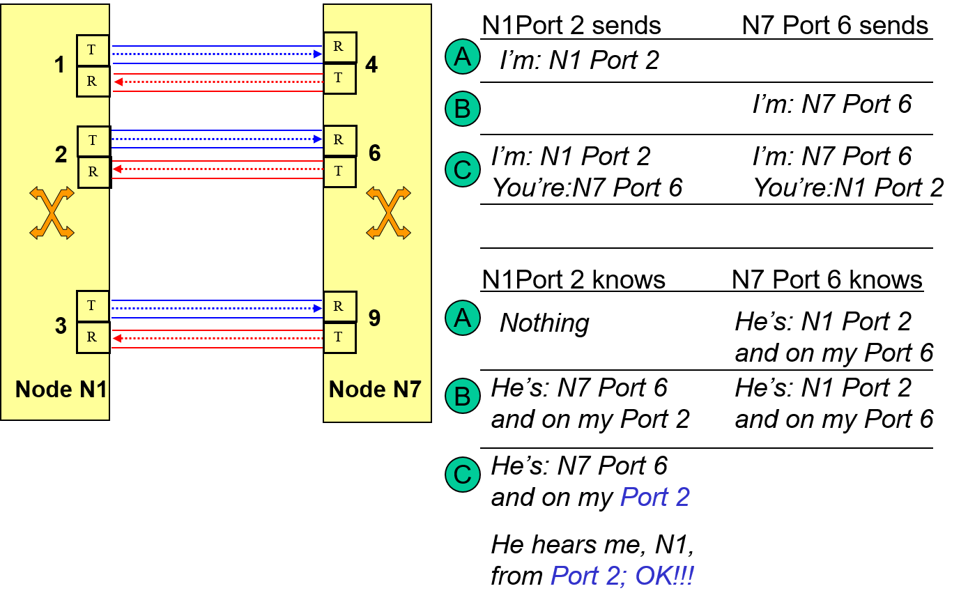
How this works in the networking world is shown in Figure 17, where each link endpoint sends some kind of message to announce its identity (e.g., like an IP address, Ethernet address, etc.) and port number. When each link endpoint has completed the full procedure it then has information about the link and its neighbor. By gathering all this link information one then obtains the complete topology of the network.

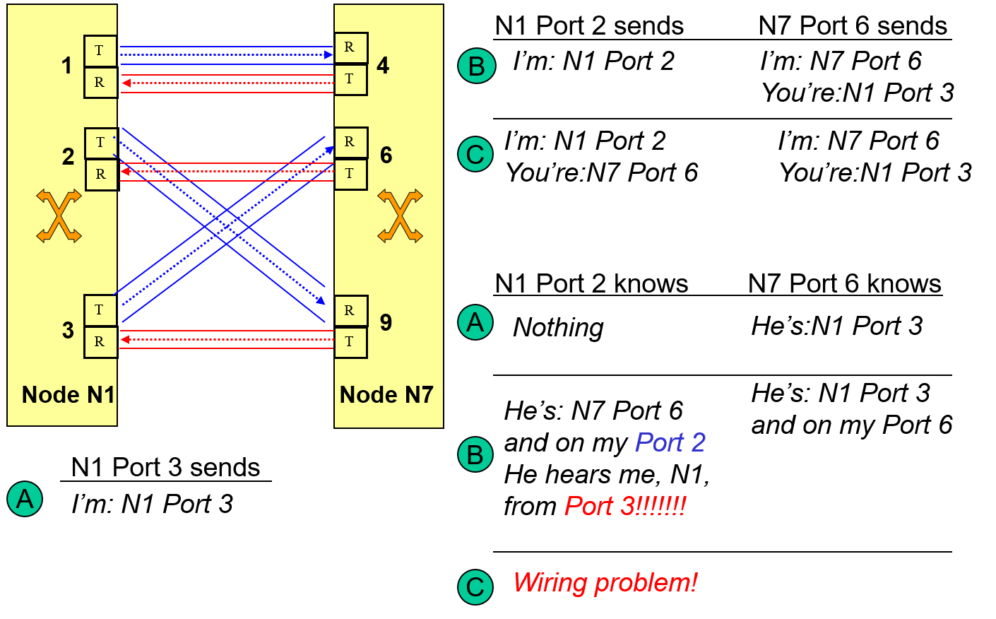
In addition to discovering a neighbor this procedure can also alert us to subtle mis-wiring problems that can occur with high fiber count systems as shown in 18 .

The first major complication for endpoint discovery in optical networks is that, unlike IP networks, optical networks are layered and not flat. Hence we have the additional question of “who’s my neighbour at layer X” as show in Figure 19. For example in the network shown layered we can speak of neighbour endpoints at the IP layer, G.709 ODUk layer, G.709 OTUk (regenerator) layer, the optical channel layer, or the optical transport (optical amplifier) layer. If router IP1 uses the hello protocol built into OSPF it will not discover its neighboring G.709 multiplexer M1, but its IP layer neighbor router IP2. Hence we will need to perform layer specific discovery, i.e., we need to "say hello" at the proper layer!

The second major difference between our optical situation and the IP situation is that in the IP case both data plane and control communications occur over the exact same “channel”. In the optical case this is not necessarily true, and hence we need to make sure that whatever mechanism used for optical discovery is applicable to the data plane. We saw two such mechanisms for the G.709 OTUk (regenerator) layer: the GCC0 (general communications channel 0) or the TTI (trail trace identifier). The concepts of multi-layer optical discovery are formalized in ITU-T G.7714. Specific techniques applicable to G.709 are given in G.7714.1. In the table below we highlight some of the "hello" protocols that are used for discovery at various networking layers.

Layer	Standard	Description
IPv4	OSPFv2	Contains a "hello" sub-protocol
IPv6	RFC4861	"Neighbor Discovery for IP version 6"
Ethernet	802.1AB	Link Layer Discovery Protocol (LLDP)
Optical	G.7714	ITU-T "Generalized Automatic Discovery"

Optical Path Computation

When dealing with high speed digital TDM signals such as G.709, despite the complexity of the multiplexing hierarchy, we can still think in terms of a particular signal component (part of the multiplex) as occupying a particular time slot. When such multiplex signals are switched we can specify the switch forwarding tables in terms of conceptual pairs of (input port, input timeslot) to (output port, output timeslot). Such an entry in a switch forwarding table is called a cross connect. We've seen these before in MPLS where they looked took the form (input port, input label) to (output port, output label). Given the MPLS control plane (OSPF-TE, RSVP-TE) you might guess that we could substitute real MPLS labels with timeslots and then be able to control high speed TDM networks and you'd be essentially correct. This idea forms the basis for Generalized Multi-Protocol Label Switching (GMPLS), i.e., the extension of the MPLS control plane to control non-packet technologies.

When we are dealing with optical networks that utilize wavelength based switches such as the ROADMs previously discussed we are presented with an additional complication. As we learned practical all optical wavelength converters do not exist and wavelength converters based on optical-electrical-optical technology are quite expensive and hence are to be avoided. This implies that when selecting a path between to end points in a transparent optical network we need to make sure that we can use the same wavelength on all links of the path. This is known as the Routing and Wavelength Assignment (RWA) problem and computational complexity wise it is quite difficult.

Consider the transparent optical network shown in Figure 20 to be used to connect data centers. Suppose the following data centers want to establish a wavelength based connection: (DC1, DC2), (DC3, DC4) and (DC1, DC5). The shortest paths between these data center pairs are listed in the table below. On the diagram we give a list of the available wavelengths on each link.

Src, Dst	Shortest Path	Length	Wavelengths
DC1, DC2	S2, S3, S4	509.5	$\lambda_1$
DC3, DC4	S3, S2, S6, S7	671.7	$\lambda_1$
DC1, DC5	S2, S6, S7, S8	639.0	$\lambda_1$

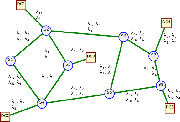
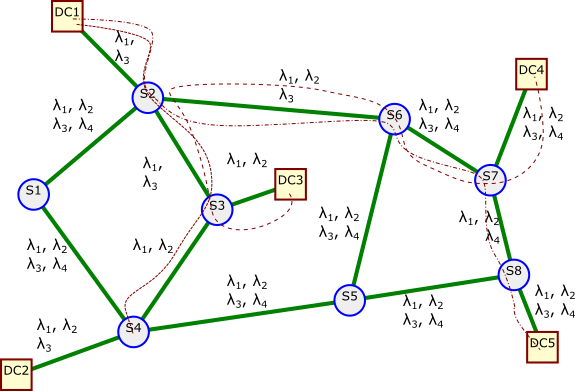
The good news is that for each of the shortest paths a wavelength is available. The bad news is that pair of these shortest paths overlap on at least one link hence we can only set up one out of three of these paths! This is problem is illustrated in Figure 21 where dashed lines are used to indicate the shortest paths and all paths have the same color since only same wavelength is available for all the paths.

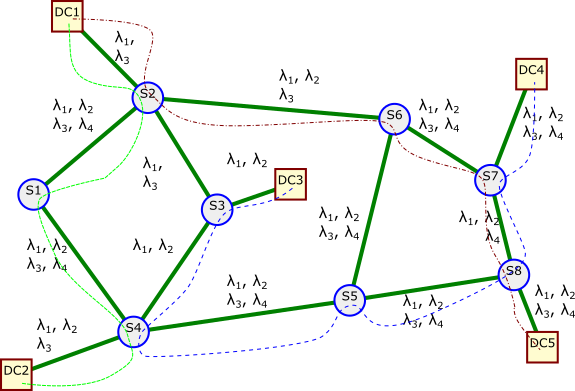
How might we fair if we considered alternative paths such as that generated by a k-shortest path algorithm. Consider the paths shown in the table below:

Path	Rank	Length	Wavelengths
DC1, S2, S1, S4, DC2	2nd	548.5	$\lambda_1, \lambda_3$
DC3, S3, S4, S5, S8, S7, DC4	2nd	806.3	$\lambda_1, \lambda_2$
DC1, S2, S6, S7, S8, DC5	1st	509.5	$\lambda_1$

If we let the path from DC1-DC5 use $\lambda_1$, the path from DC1-DC2 use $\lambda_3$, and the path from DC3-DC4 use $\lambda_2$ we have no collisions where these paths overlap. This is shown diagramatically in Figure 22 where we show the paths via dashed lines and represent different wavelength assignments by the different colors of the paths. Note that how on any link where the the paths overlap the colors of the paths are different!

Topology Aggregation and Dissemination

We can extract neighbor and link information learned through a discovery process to a central controller or management system. Another approach would be to distribute this information to all the nodes in the network as is done in link state IP routing protocols. As a review link state IP routing protocols contain the following categories of functionality:

• Discovery portion

  Uses a Hello protocol with the assumption that data and control planes the same. We just learned that more general techniques are needed for optical and other multilayer networks. Hence, this functionality in general, is not applicable to optical networks.

• Topology dissemination

  Information concerning nodes (including reachability) and links in the network is distributed to all nodes via very efficient update procedures for use in path computation. We need much more information to enable path computation in optical networks.

• Route computation

  Is included in link state routing protocols to construct IP forwarding tables. Such computations are heavily constrained due to hop by hop (destination based) forwarding paradigm. These procedures are overly simplistic for optical path computations and limit very important alternative paths.

As the above list shows for the purpose of an optical control plane the topology dissemination portion of link state routing protocols is of prime interest. Analogous to what was done to enable MPLS traffic engineering where link bandwidth information was added to OSPF's link state advertisements (LSAs) we can add information needed for optical path computation too. We give two examples of such information: link wavelength availability and node connectivity constraints.

Wavelength Availability

The first thing we need is a way to describe wavelengths. Wavelengths can be considered a "generalized" label, i.e., we use it to identify the signal of interest within a multiplex. This idea lead to the term "Generalized MPLS" (GMPLS) for the extension of the MPLS control plane for use with optical networks.

Such "wavelength labels" are defined in RFC6205 based on the ITU-T G.694.1 dense and coarse WDM grids (DWDM and CWDM).

The DWDM grid is based on specific center frequencies given by:

Central Frequency (THz) = 193.1 THz + n * channel spacing (THz)

Where "n" is an integer (positive, negative, or 0) and "channel spacing" is defined to be 0.0125, 0.025, 0.05, or 0.1 THz.

This gets encoded into a label as shown below:

    0                   1                   2                   3
    0 1 2 3 4 5 6 7 8 9 0 1 2 3 4 5 6 7 8 9 0 1 2 3 4 5 6 7 8 9 0 1
   +-+-+-+-+-+-+-+-+-+-+-+-+-+-+-+-+-+-+-+-+-+-+-+-+-+-+-+-+-+-+-+-+
   |Grid | C.S.  |    Identifier   |              n                |
   +-+-+-+-+-+-+-+-+-+-+-+-+-+-+-+-+-+-+-+-+-+-+-+-+-+-+-+-+-+-+-+-+

Where "Grid" indicates whether the DWDM or CWDM grid is used, "C.S." indicates the channel spacing, "Identifier" is optional, and "n" is a 16-bit two's complement representation of the integer n from the center frequency formula.

In order to compute optical paths we need to know wavelength availability, and for transparent optical networks we need to know exactly which wavelengths are available. We could send a list of available wavelengths, since this information could be updated frequently a more efficient method is also desirable. Most DWDM systems have channel counts in the 10 to 120 range. Since this is relatively low we could represent an available channel by a bit in a "bit map". This is done in RFC7579 in their "bitmap label set" as shown below:

      0                   1                   2                   3
      0 1 2 3 4 5 6 7 8 9 0 1 2 3 4 5 6 7 8 9 0 1 2 3 4 5 6 7 8 9 0 1
     +-+-+-+-+-+-+-+-+-+-+-+-+-+-+-+-+-+-+-+-+-+-+-+-+-+-+-+-+-+-+-+-+
     |  4    |   Num Labels          |             Length            |
     +-+-+-+-+-+-+-+-+-+-+-+-+-+-+-+-+-+-+-+-+-+-+-+-+-+-+-+-+-+-+-+-+
     |                         Base Label                            |
     |                            . . .                              |
     +-+-+-+-+-+-+-+-+-+-+-+-+-+-+-+-+-+-+-+-+-+-+-+-+-+-+-+-+-+-+-+-+
     |    Bitmap Word #1 (Lowest numerical labels)                   |
     +-+-+-+-+-+-+-+-+-+-+-+-+-+-+-+-+-+-+-+-+-+-+-+-+-+-+-+-+-+-+-+-+
     :                                                               :
     +-+-+-+-+-+-+-+-+-+-+-+-+-+-+-+-+-+-+-+-+-+-+-+-+-+-+-+-+-+-+-+-+
     |    Bitmap Word #N (Highest numerical labels)                  |
     +-+-+-+-+-+-+-+-+-+-+-+-+-+-+-+-+-+-+-+-+-+-+-+-+-+-+-+-+-+-+-+-+

Where "Num Labels" tells us the number of labels represented bythe bitmap. Each bit in the bitmap represents a particular label with a value of 1/0 indicating whether or not the label is in the set. Bit position zero represents the lowest label and corresponds to the base label, while each succeeding bit position represents the next label logically above the previous.

Asymmetric Switches

When we learned about one of the most prevalent forms of optical switching, the ROADM, we also saw that it was quite different from most packet or electronic circuit switches in that the signals from some input ports could not reach all output ports. This represents a significant node constraint that needs to be taken into account when automating optical path computation. A very straight forward way to model this is via a "potential" connectivity matrix as shown in figure 23 .

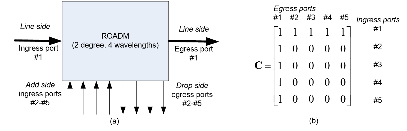
An efficient encoding for this connectivity matrix is given in RFC7579 section 2.1 and is shown below.

       0                   1                   2                   3
       0 1 2 3 4 5 6 7 8 9 0 1 2 3 4 5 6 7 8 9 0 1 2 3 4 5 6 7 8 9 0 1
      +-+-+-+-+-+-+-+-+-+-+-+-+-+-+-+-+-+-+-+-+-+-+-+-+-+-+-+-+-+-+-+-+
      | Conn  |   MatrixID    |            Reserved                   |
      +-+-+-+-+-+-+-+-+-+-+-+-+-+-+-+-+-+-+-+-+-+-+-+-+-+-+-+-+-+-+-+-+
      |                         Link Set A #1                         |
      :                               :                               :
      +-+-+-+-+-+-+-+-+-+-+-+-+-+-+-+-+-+-+-+-+-+-+-+-+-+-+-+-+-+-+-+-+
      |                         Link Set B #1                         :
      :                               :                               :
      +-+-+-+-+-+-+-+-+-+-+-+-+-+-+-+-+-+-+-+-+-+-+-+-+-+-+-+-+-+-+-+-+
      |                 Additional Link Set Pairs as Needed           |
      :                     to Specify Connectivity                   :
      +-+-+-+-+-+-+-+-+-+-+-+-+-+-+-+-+-+-+-+-+-+-+-+-+-+-+-+-+-+-+-+-+

Signaling/Light Path Management

As in the MPLS case we can set up the needed cross-connection for a (real or virtual) circuit via a management system or a signaling protocol. If we use a signaling protocol we will want to be able to specify the specific path that we want taken between source and destination. In the case of transparent optical networks we may need to specify the wavelength to be used. Our signaling protocol will send a "setup" message down the specified path requesting resouces (timeslots or wavelengths) enabling switches to set up the required cross-connects. In wavelength and TDM switching wavelengths or time slots become our "virtual labels" and allow us to extend protocols developed for use with MPLS.

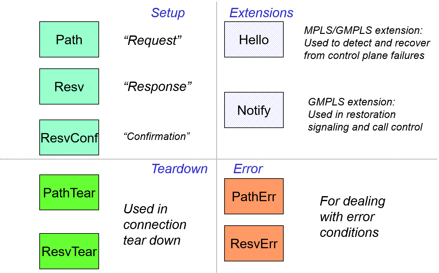
RSVP-TE (resource reservation protocol-traffic engineering) is such a signaling protocol and provides for the explicit designation of the path to be taken by the circuit. Remember that LDP (Label Distribution Protocol) could only set up LSPs (label switched paths) along paths taken by IP packets. Hence RSVP-TE is the main signaling protocol used in GMPLS. By the time it was used in GMPLS it already had quite a long heritage. This tends to make it difficult to understand without providing some translation into more common terminology. In Figure 24 we show the RSVP-TE messages used in the setup and teardown of circuits as well as extensions and error processing.

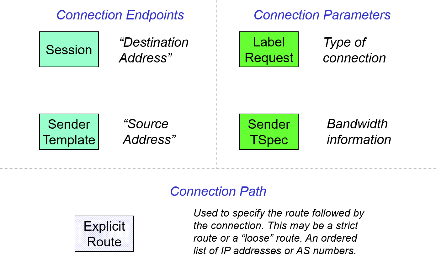
In Figure 25 we show the "objects" used in an RSVP-TE path message and their purpose. Once again the strange RSVP-TE terminology shown in the boxes in the figure stems from RSVP-TE long history and initial start as a very general reservation protocol rather than a traffic engineering oriented protocol.

With all the added complexity that a signaling protocol brings you might wonder why you would want to use one in an optical network. A centralized controller is generally better at path computation and network optimization, in optical networks the rate of connection setup/teardown will generally not be large, i.e., these are very high capacity circuits, whose useage would tend to change slowly, at most with day/night cycles rather than on minute or second time scales. Under these circumstances a central controller would not been a connection setup/teardown bottleneck.

However, there is one very import general situation where a central can become a bottleneck and that is during network failure/restoration events. Long haul and metro optical networks due to there high capacity have had fairly strict reliability requirements. Standardized linear and ring protection schemes have restoration times of less than 60 mS! These schemes can be wasteful of network bandwidth, if more time is given much more bandwidth efficient restoration schemes can be implemented and GMPLS signaling forms the basis of many schemes used in carrier networks that can restore sevices in less than 2 seconds.

References

Recommended Readings

RFC6163 Framework for GMPLS and Path Computation Element (PCE) Control of Wavelength Switched Optical Networks (WSONs), Y. Lee, G. Bernstein, W. Imajuku, 2011.

Read sections: 3.1-3.6 (skip 3.6.1)

ITU-T Handbook: http://www.itu.int/dms_pub/itu-t/opb/hdb/T-HDB-OUT.10-2009-1-PDF-E.pdf  Lots of good information, a great free 324 page reference. Browse. Do not read line by line.

IEEE 802.3-2012 Section 6 Chapters 80-89 on 40Gbps and 100Gbps Ethernet. Browse. Do not read line by line.

ITU-T Recommendation G.709, 12/2009. Browse. Do not read line by line.

Optional Readings

RFC6566 A Framework for the Control of WSONs with Impairments, March 2012. More information on how impairments can be handled in the control plane.

G. M. Bernstein, Y. Lee, A. Gavler, and J. Martensson, Modeling WDM Wavelength Switching Systems for Use in GMPLS and Automated Path Computation, Journal of Optical Communications and Networking , vol. 1, no. 1, pp. 187-195, Jun. 2009.