Introduction

In the following we describe a modern practical technique for network modeling and visualization. The modeling methods discussed here are intended for network education, research, and optimization. They are not intended as a replacement for network management modeling languages such as YANG. The goal here is to minimize the amount of time spent on learning to model a network by keeping the modelling methodology as simple as possible while also supporting nearly arbitrary extensions modern libraries and tools.

All the models for network related entities given below are implemented with JavaScript Object Notation JSON. JSON is a standard, text based, data exchange format which is easy for both humans and machines to process and is supported (internally or via external libraries) by almost all programming languages. To formalize and validate our models we use JSON schemas. However, users can safely ignore the formal schema and just follow the given examples or the output from the example code on this website or from our communications network visualization (ComNetViz) web app.

Visualization with SVG

To visualize networks and their associated entities such as paths, user demands, link bandwidth, etc. we utilize the Scalable Vector Graphics (SVG) standard supported by all modern web browsers. This graphics format is preferable to GIF, PNG, or JPG in that individual graphic objects within a figure can be styled or manipulated (with the help of CSS or JavaScript). For example in Figure @fig:NetworkSVG the path {N2, N4, N5, N6} was highlighted in red just by changing an SVG class attribute on the links of interest and setting the color for those "highlighted" links via Cascading Style Sheets (CSS). This network is used on another page to illustrate the "scheduled backup" combined network/compute optimization problem.

{#fig:NetworkSVG width=600px}

JSON Network Models

The JSON network format we use to save and share network models is based on that used in the NetworkX open source Python graph library. NetworkX provides a wide variety of very useful graph data structures and algorithms as well graph I/O facilities. Important Note: this format we use here and used by NetworkX has changed! We have moved to new format described below and compatible with NetworkX 2.x as of 2018.

In code fragment 1 we show the JSON representation for a network consisting of nodes named [N1, N2, N3, N4] connected by the links (N1, N2), (N2, N4), (N3, N4). We see that the representation consists of a list of nodes and a list of links. One subtle aspect of the NetworkX representation is that the "source" and "target" attributes for a link is given by the position of the corresponding node in the "nodes" array and not by the node's identifier.

{
    "directed": false,
    "graph": {},
    "nodes": [
        {"id": "N1"},
        {"id": "N2"},
        {"id": "N3"},
        {"id": "N4"}
    ],
    "links": [
        {"source": "N1", "target": "N2"},
        {"source": "N2", "target": "N4"},
        {"source": "N3", "target": "N4"}
    ],
    "multigraph": false
}

Code Fragment 1. Minimal JSON graph representation.

To model and draw networks we typically want to associate more information with nodes and links. For the network shown in Figure 1 we need (x, y) coordinates for each node, the node type, e.g., data center or switch. For the links in Figure 1 we want capacity and weight parameters. In addition, since this network is used to specify a network/compute optimization problem, we added problem specific data such as cost or demand associated with a data center. In code fragment 2 we show how these node and link attributes can be added to the JSON representation.

{
  "directed": false,
  "multigraph": false,
  "graph": {"name": "Figure1JSON",
       "desc": "This is the JSON used to produce Figure 1."},
  "nodes": [
    {"y": 172, "x": 573, "type": "switch", "id": "N7"},
    {"y": 188.6, "x": 71, "type": "data_center", "id": "DC0", "demand": 237},
    {"y": 365.6, "x": 109, "type": "data_center", "id": "DC1", "demand": 380},
    {"y": 63.7, "x": 486, "type": "data_center", "id": "DC4", "cost": 50},
    {"y": 394.6, "x": 489, "type": "data_center", "id": "DC6", "cost": 20},
    {"cost": 70, "y": 324.6, "x": 261, "type": "data_center", "id": "DC3"},
    {"y": 409.4, "x": 311, "type": "switch", "id": "N8"},
    {"y": 80.6, "x": 432, "type": "switch", "id": "N9"},
    {"y": 338, "x": 526, "type": "switch", "id": "N6"},
    {"y": 108.6, "x": 230, "type": "switch", "id": "N0"},
    {"y": 235, "x": 61, "type": "switch", "id": "N1"},
    {"y": 315, "x": 74, "type": "switch", "id": "N2"},
    {"y": 304, "x": 309, "type": "switch", "id": "N3"},
    {"y": 208, "x": 337, "type": "switch", "id": "N4"},
    {"y": 215, "x": 467, "type": "switch", "id": "N5"},
    {"cost": 60, "y": 170.6, "x": 468, "type": "data_center", "id": "DC5"},
    {"demand": 220, "y": 166.6, "x": 248, "type": "data_center", "id": "DC2"}],
  "links": [
    {"source": "N7", "capacity": 50, "target": "N9", "weight": 133.1},
    {"source": "N7", "capacity": 50, "target": "N6", "weight": 143.6},
    {"source": "DC0", "capacity": 50, "target": "N1", "weight": 91.3},
    {"source": "DC1", "capacity": 50, "target": "N2", "weight": 100.8},
    {"source": "DC4", "capacity": 50, "target": "N9", "weight": 95.3},
    {"source": "DC6", "capacity": 50, "target": "N6", "weight": 73.5},
    {"source": "DC3", "capacity": 50, "target": "N3", "weight": 47.1},
    {"source": "N8", "capacity": 50, "target": "N2", "weight": 223.7},
    {"source": "N8", "capacity": 50, "target": "N3", "weight": 68.1},
    {"source": "N8", "capacity": 50, "target": "N6", "weight": 186.2},
    {"source": "N9", "capacity": 50, "target": "N0", "weight": 159.6},
    {"source": "N9", "capacity": 50, "target": "N4", "weight": 119.3},
    {"source": "N6", "capacity": 50, "target": "N5", "weight": 109.2},
    {"source": "N0", "capacity": 50, "target": "N1", "weight": 179.7},
    {"source": "N0", "capacity": 50, "target": "DC2", "weight": 80.3},
    {"source": "N1", "capacity": 50, "target": "N2", "weight": 56.3},
    {"source": "N2", "capacity": 50, "target": "N4", "weight": 250},
    {"source": "N3", "capacity": 50, "target": "N4", "weight": 74.4},
    {"source": "N4", "capacity": 50, "target": "N5", "weight": 103.2},
    {"source": "N5", "capacity": 50, "target": "DC5", "weight": 30}]
}

Code Fragment 2. JSON graph representation for the network of Figure 1.

The nice thing about JSON and the NetworkX JSON network representation is that we can add arbitrary attributes to the nodes and links in a network and these extra attributes can be used or ignored in any subsequent processing. Below we summarize various attributes that we currently use in our network modelling and associated algorithms. For more detail see the examples, in addtion our formal network JSON-schema can be found in the file netSchema.json.

• Node Attributes

  • id: (required) a name for the node, must be unique in the network.
  • x, y: coordinates of the node (required for drawing network)
  • type: (optional) Currently defined types are "switch", "host", "data_center", "user_region". These are mostly used by algorithms to differentiate different types of nodes, e.g., assign IPv4 addresses only to hosts, they are also used in visualization by drawing different shapes for different node types.
  • layer: (optional) the layer that the node is operating at. Used in modeling multi-layer networks, e.g., IP over Optical, for optimization and path computation. In the web app we support "none", "ip", "ether", "sdh", "g709", "wavelength" respectively representing No layer information, IP, Ethernet, SONET/SDH, G.709, and Wavelength layers. In visualization when both ends of a link are at a given layer we assign a specific color to that link. When a link is between nodes at different layers we use a dotted line to represent the link as sometimes done in ITU-T diagrams.
  • ipv4: (optional) an IPv4 address assigned to the node. Useful when models are used with emulators such as Mininet.
  • mac: (optional) an Ethernet (MAC) address assigned to the node. Useful when models are used with emulators such as Mininet.

• Link Attributes

  • source, target: (required) the source and target node ids.
  • capacity: (optional) Indicates the capacity of the link. Visualization tools can use this to enhance an SVG drawing.
  • weight: (optional) Typically used by path computation and optimization algorithms.
  • ports: (optional) This indicates the ports used by this link on both source and target nodes. This information is needed by algorithms that construct/fill forwarding tables in switches and can also be useful when constructing networks in emulators.

• General Network/Graph Attributes

  • name: (optional) Useful in telling networks apart. Our web app currently displays this.
  • desc: (optional) Useful in reminding yourself and the rest of the world what this network model was for.

JSON Network Demand Representation

For some network optimization problems we start with a set of traffic demands between network nodes. Such demands can easily be represented via JSON as shown in code fragment 3. In Figure @fig:NetwDemands we show a visualization of these demands on an extremely simplistic network. The demands are shown via grey lines between nodes. In this visualization the thickness of the demand lines and the links is roughly proportional to the demands between the nodes and the link capacity respectively. The JSON for this network is given in code fragment 4.

{   "id": "DemandEx1",
    "desc": "Example of demand JSON format",
    "demandList":
        [
            {"source": "N2", "target": "N0", "demand": 40.0},
            {"source": "N3", "target": "N1", "demand": 35.0},
            {"source": "N1", "target": "N3", "demand": 35.0},
            {"source": "N0", "target": "N2", "demand": 40.0}
        ]
}

Code Fragment 3. JSON demand representation for the simple network of Figure 2.

{#fig:NetwDemands width=500px}

{
    "directed": false,
    "multigraph": false,
    "graph": {"name": "demandExampleNet",
              "desc": "Network to demonstrate demand format"},
    "nodes": [
        {"y": 50, "x": 173, "id": "N0"},
        {"y": 260, "x": 183, "id": "N1"},
        {"y": 254, "x": 538, "id": "N2"},
        {"y": 17, "x": 503, "id": "N3"},
        {"y": 87, "x": 323, "id": "N4"}
    ],
    "links": [
        {"source": "N0", "capacity": 45, "target": "N1", "weight": 10},
        {"source": "N0", "capacity": 50, "target": "N3", "weight": 10},
        {"source": "N0", "capacity": 40, "target": "N4", "weight": 7},
        {"source": "N1", "capacity": 42, "target": "N2", "weight": 15},
        {"source": "N1", "capacity": 45, "target": "N4", "weight": 10},
        {"source": "N2", "capacity": 30, "target": "N3", "weight": 12}
    ]
}

Code Fragment 4. JSON representation for the extremely simple network of Figure 2.

As shown in Figure @fig:DemandDialog sortable tables are useful for visualizing demands. The JSON schema for our demand format is available in the file demandSchema.json.

{#fig:DemandDialog width=400px}

JSON Path Representations

The output of many network optimization algorithms includes a path or a set of paths. Visualizing these paths can be key to understanding and/or verifying an optimization or algorithm. The key information about a path is the sequence of nodes that it traverses. Hence the key element in our JSON model for paths is a path list (pathList) and within each path in the list we have a list of nodes (nodeList). This can be seen in an example of our JSON based path model shown in code fragment 5.

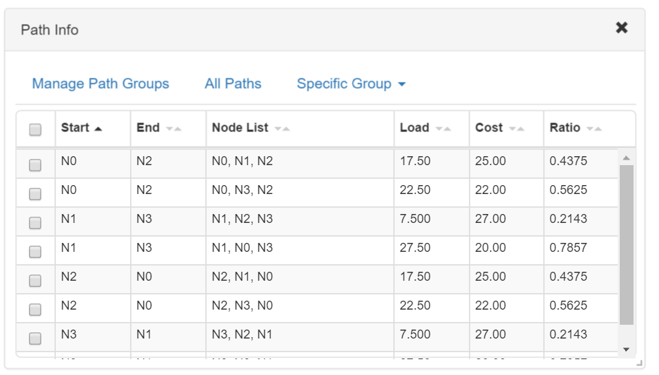
Depending on the algorithm that generated the path set one may want to keep other information with each path. The paths in code fragment 5 were the outcome of a batch network optimization procedure known as a multi-commodity flow problem. In this problem we seek to find multiple paths between various source and destinations that will satisfy the communications demands within the bandwidth constraints of the links and with over all minimum cost. Hence, the JSON path representation of code fragment 5 includes a cost, load, and ratio information for each path. The "ratio" information is the percentage of the overall demand traffic between two nodes carried by the path.

In Figure @fig:PathTable we show a screen capture of a dialog box from our web app used to sort and select paths for visualization based on this information. Note that in networks with parallel links, i.e., a multigraph, one would need to identify specific links rather than a list of nodes. However we currently model parallel links as an aggregated link (like Ethernet link aggregation groups) rather than using a multi-graph. The JSON-schema for our path format is available in the file pathSchema.json.

{   "id": "PathsEx1",
    "desc": "Example paths compatible with the demandExampleNet network",
    "pathList": [
        {"load": 17.5, "nodeList": ["N2", "N1", "N0"], "cost": 25, "ratio": 0.4375},
        {"load": 22.5, "nodeList": ["N2", "N3", "N0"], "cost": 22, "ratio": 0.5625},
        {"load": 7.5, "nodeList": ["N1", "N2", "N3"], "cost": 27, "ratio": 0.2143},
        {"load": 27.5, "nodeList": ["N1", "N0", "N3"], "cost": 20, "ratio": 0.7857},
        {"load": 7.5, "nodeList": ["N3", "N2", "N1"], "cost": 27, "ratio": 0.2143},
        {"load": 27.5, "nodeList": ["N3", "N0", "N1"], "cost": 20, "ratio": 0.7857},
        {"load": 17.5, "nodeList": ["N0", "N1", "N2"], "cost": 25, "ratio": 0.4375},
        {"load": 22.5, "nodeList": ["N0", "N3", "N2"], "cost": 22, "ratio": 0.5625}]
}

Code Fragment 5. JSON representation a set of paths with extra information specific to an optimization problem.

{#fig:PathTable width=400px}

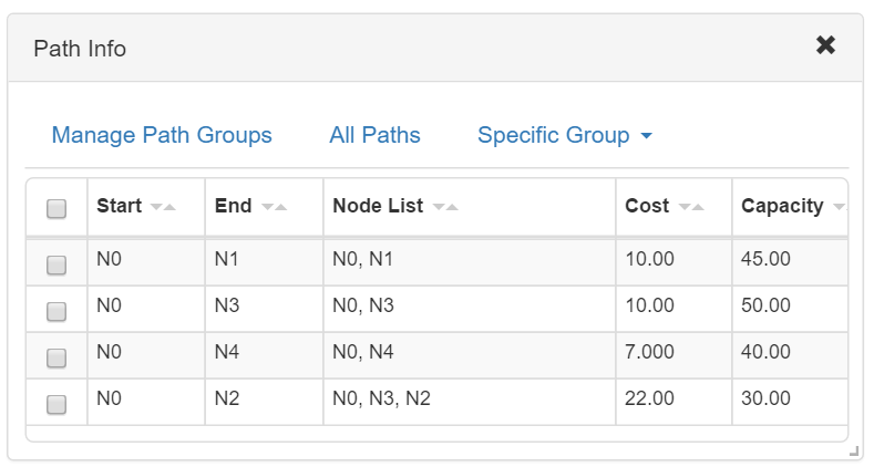
In code fragment 6 and Figure @fig:PathTable2 we show a group of paths with a different set of additional attributes. These paths were the result of a shortest path computation and include the path cost and capacity. This shows again how JSON makes it easy to give a path any useful attributes. In addition, our web app (ComNetViz) will pick up arbitrary path attributes and show them in a path table.

{ "id": "Shortest_N0_All",
  "desc": "Shortest paths from node N0",
  "pathList": [
    {"cost": 10, "capacity": 45, "nodeList": ["N0", "N1"]},
    {"cost": 10, "capacity": 50, "nodeList": ["N0", "N3"]},
    {"cost": 7,  "capacity": 40, "nodeList": ["N0", "N4"]},
    {"cost": 22, "capacity": 30, "nodeList": ["N0", "N3", "N2"]} ]
}

Code Fragment 6. JSON representation of a set shortest paths with extra information on path cost and capacity.

{#fig:PathTable2 width=400px}

Examples/Web App

We encourage readers to give our web based "beta" communications network editor/visualizer ComNetViz a try. You can copy and paste any of the above network, demand, or path JSON models into ComNetViz or see below for more example network and path files.

1. Simple Network and Paths
   1. Simple network model
   2. Paths for simple network
2. Network with link port assignments, IPv4 addresses, and MAC addresses for the hosts ExNetwithLoops1B.json
3. Multi-layer example network model
4. Network for a medium sized ficticious country with Paths
   1. Medium network model
   2. Paths for medium network
5. Large network example (54 nodes 102 links)
   1. Network model JSON
   2. Disjoint path pairs

A Simple Computation Server

We've shown how to model and visualize networks and various network related entities such as demands, paths, etc... and with our ComNetViz web app you can visualize the results of your network computations by either opening a JSON file or just load JSON strings into the application. However, for evaluating many test cases or for frequent updates it would be nice for the visualization system (browser) to talk directly to a computation server. In the "old days" a network student or researcher wouldn't never want to bother with the complexity of a client-server system, in this section we show how it can be done relatively easily with Python on the server side and our existing ComNetViz web app.

The ComNetViz app has just a few built in computation algorithms: (a) shortest paths (Dijkstra), (b) minimum spanning tree (Prim), and (c) widest paths (modified Dijkstra). A very useful path computation algorithm for network planning/optimization is a k-shortest path algorithm (finds not just the shortest but the 2nd shortest, 3rd shortest, ... k shortest path between two nodes). There are multiple algorithms in the literature for computing the k-shortest paths, however none of them are simple and although I've implemented one of these in Python, my code is not nearly as fast or general as the k-shortest path algorithm now available in the NetworkX Python graph library. Hence in this section we will show the techniques needed for a client-server based approach to k-shortest paths with nice web browser based visualization of the results.

The Key interface and implementation ingredients are:

1. A standard method for Browser and Server to communicate — the simplest and most widely available technique for this is known as AJAX. AJAX allows sending and receiving computation requests without changing web pages. We use the relatively new FetchAPI in our ComNetViz app.

   An alternative approach that would be good for dealing with longer lived optimization computations that produce intermediate results and that may need to be stopped/restarted would be Websockets, but we don't need this added functionality and the complexity that comes with it for our k-shortest path computation.

2. A Server interface methodology — Here we will borrow from current web practices and use a REST like interface along with JSON to carry information back and forth. The key REST aspect that we will be concerned with is that of using different URLs to identify different types of computation requests. We'll show a "test" interface as well as our k-shortest path interface below.

3. A Server implementation via the Flask Python micro-framework. The Flask framework greatly simplifies the server implementation. Since we will want the compute server to run on a separate machine, i.e., you machine, than the ComNetViz app (this website) we need to enable a web feature known as cross origin resource sharing CORS. We do this via the flask CORS library.

The complete server implementation is available in the file computeServer.py. The file is less than 120 line long. To run it you will need a Python installation along with the Flask, Flask-CORS, and NetworkX libraries installed. In code fragment 7 we show the key parts of our server implementation enabled by Flask and NetworkX. Some key points to this code are:

• On lines 1 and 9 of the snippet a Python decorator is used to associate trailing part of a URL (and HTTP methods) with the function that follows on the next line (lines 2 and 10).
• On lines 3 and 11 we use a Flask request object to get the JSON data sent to the server from the web browser.
• For the k-shortest path computation on lines 12-15 we extract from the JSON the network, source and destination nodes, and the number k of paths to compute. Note that line 12 gets the network from the JSON and then uses a NetworkX function to convert it to NetworkX's native Python format which is computationally efficient.
• On lines 16 and 17 we call the NetworkX function that computes the k-shortest paths. Note that the NetworkX k-shortest paths function (shortest_simple_paths) uses a Python technique called generators to be efficient and general hence the extra stuff on line 17.
• On line 18 we call a function to take the results from the algorithms and add more information to the paths such as cost and capacity. The createPathsInfo() function is included in the server file.
• Finally on lines 19 and 20 we prepare an identifier for the path group and a description and on line 21 we call the Flask jsonify() function to convert from our Python to JSON which then gets sent to the client (Browser).

@app.route('/test', methods=['POST', 'GET'])
def test():
    testJSON = request.get_json()
    print(testJSON)
    return jsonify(server="My Local Server", capabilities=capabilities,
                   echo=testJSON)


@app.route('/kShortestPaths', methods=['PUT', 'POST'])
def k_shortest_paths():
    kshortPathProb = request.get_json()
    net = json_graph.node_link_graph(kshortPathProb["net"])
    srcNode = kshortPathProb["srcNode"]
    dstNode = kshortPathProb["dstNode"]
    k = int(kshortPathProb["k"])
    pathGen = shortest_simple_paths(net, srcNode, dstNode, weight="weight")
    paths = list(islice(pathGen, k))
    pathsInfo = createPathsInfo(paths, net)
    path_id = "kShortestPaths-" + srcNode + "-" + dstNode
    desc = "Shortest Paths from node " + srcNode + " to node " + dstNode
    return jsonify(id=path_id, desc=desc, pathList=pathsInfo)

Code Fragment 7. Python snippet of the essential k-shortest path server functionality.

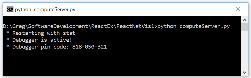
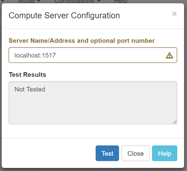
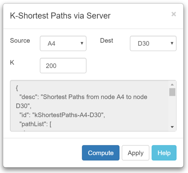
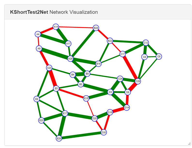
To put our server to work we need to run the computeServer.py code on a machine somewhere as shown in Figure @fig:ServerRun. To do this we use the command python computeServer.py. In the ComNetViz web app we then use the configure server dialog show in Figure @fig:ComputeTestDialog to set the name/address of the server and the port number. In Figure @fig:kPathDialog we show the dialog box used to send a request to the server to compute the 200 shortest paths between nodes A4 and D30 in our medium sized sample network. Finally in Figure @fig:kPathResult we visualize the shortest path and the 200th shortest path.

{#fig:ServerRun width=500px}

{#fig:ComputeTestDialog width=400px}

{#fig:kPathDialog width=400px}

{#fig:kPathResult width=400px}