Page Contents
Data Center Schedule Backup
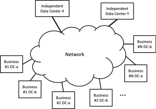
In Figure 1, we show multiple data centers connected to a network. In this scenario, data center $D{C_s}$ needs to do a bulk transfer of data to one or more remote data centers, $D{C_r}$, within prescribed time limits. In particular there ${Q_s}$ is bytes of data to be transferred between $D{C_s}$ and the set of possible remote data centers ${\bf{D}}{{\bf{C}}_r}(s)$, and the data transfer must start by time $Star{t_s}$ and end before time $En{d_s}$.
Let $rate_t^{sr}$ denote the rate that $D{C_s}$ is transferring data to $D{C_r}$ during time period $t = 0,1,...,T$. Here we break down the time interval over which scheduling is to occur, e.g., 24 hours, into a fixed number of equally spaced periods of length $\tau$ in time. The requirement that all the data must be transferred can be expressed as $$\sum\limits_{r \in {\bf{D}}{{\bf{C}}_{\bf{r}}}(s)} {\tau \sum\limits_t {rate_t^{sr}} } = {Q_s}\quad \forall s $$
Suppose that each remote data center imposes a storage cost of $storageCos{t_r}$ regardless of when the transfer starts or stops, then a simple linear objective function could be: $$\alpha \sum\limits_r {storageCos{t_r}\tau \sum\limits_{s,t} {rate_t^{sr}} } + \sum\limits_{sr,t} {networkCost(rate_t^{sr},t)} $$
Where the parameter $\alpha \ge 0$ in equation (1.6) can be used to emphasize or de-emphasize the relation of storage costs to networking costs. A more realistic objective function could include a sum of (non-linear) monotonically decreasing functions of the transfer rates to encourage faster transfers as suggested in 1.
To fully specify this network/compute optimization problem we need to include the network costs and constraints from one of our two different multi-commodity flow formulations.
Scheduled Backup Example
In Figure 2 we show an example network with data centers DC0-DC6. In this problem data centers DC0-DC2 must backup their critical data and in the "problem information dialog" in the node table the particular demand is shown (typical units could be TB, Link capacities would be in units of 4TB/hour ~ 10Gbps).

In addition to increase reliability using geographic diversity these data centers are restricted in which other data centers they can backup their data. In particular: DC0 can only use DC3, DC5, or DC6; DC1 can only use DC4 or DC6; and DC2 can only use DC5 or DC6. With this additional restriction we combined the forumlation above with our multi-commodity flow given paths formulation.
The problem information including storage costs of backup data centers is given in the JSON network file shown below:
{
  "directed": false,
  "graph": { "name": "Backup Graph", "desc": "Data Center Backup Example graph" },
  "nodes": [
    { "y": 304, "x": 309, "type": "switch", "id": "N3" },
    { "y": 166.6, "x": 248, "type": "data_center", "id": "DC2", "demand": 220 },
    { "y": 315, "x": 74, "type": "switch", "id": "N2" },
    { "y": 215, "x": 467, "type": "switch", "id": "N5" },
    { "y": 409.4, "x": 311, "type": "switch", "id": "N8" },
    { "y": 80.6, "x": 432, "type": "switch", "id": "N9" },
    { "y": 170.6, "x": 468, "cost": 60, "type": "data_center", "id": "DC5" },
    { "y": 108.6, "x": 230, "type": "switch", "id": "N0" },
    { "y": 338, "x": 526, "type": "switch", "id": "N6" },
    { "y": 394.6, "x": 489, "cost": 20, "type": "data_center", "id": "DC6" },
    { "y": 235, "x": 61, "type": "switch", "id": "N1" },
    { "y": 63.7, "x": 486, "cost": 50, "type": "data_center", "id": "DC4" },
    { "y": 172, "x": 573, "type": "switch", "id": "N7" },
    { "y": 208, "x": 337, "type": "switch", "id": "N4" },
    { "y": 324.6, "x": 261, "cost": 70, "type": "data_center", "id": "DC3" },
    { "y": 188.6, "x": 71, "type": "data_center", "id": "DC0", "demand": 237 },
    { "y": 365.6, "x": 109, "type": "data_center", "id": "DC1", "demand": 380 }
  ],
  "links": [
    { "source": "N3", "capacity": 50, "target": "N8", "weight": 68.1 },
    { "source": "N3", "capacity": 50, "target": "N4", "weight": 74.4 },
    { "source": "N3", "capacity": 50, "target": "DC3", "weight": 47.1 },
    { "source": "DC2", "capacity": 50, "target": "N0", "weight": 80.3 },
    { "source": "N2", "capacity": 50, "target": "N8", "weight": 223.7 },
    { "source": "N2", "capacity": 50, "target": "N1", "weight": 56.3 },
    { "source": "N2", "capacity": 50, "target": "N4", "weight": 250 },
    { "source": "N2", "capacity": 50, "target": "DC1", "weight": 100.8 },
    { "source": "N5", "capacity": 50, "target": "DC5", "weight": 30 },
    { "source": "N5", "capacity": 50, "target": "N4", "weight": 103.2 },
    { "source": "N5", "capacity": 50, "target": "N6", "weight": 109.2 },
    { "source": "N8", "capacity": 50, "target": "N6", "weight": 186.2 },
    { "source": "N9", "capacity": 50, "target": "N0", "weight": 159.6 },
    { "source": "N9", "capacity": 50, "target": "DC4", "weight": 95.3 },
    { "source": "N9", "capacity": 50, "target": "N4", "weight": 119.3 },
    { "source": "N9", "capacity": 50, "target": "N7", "weight": 133.1 },
    { "source": "N0", "capacity": 50, "target": "N1", "weight": 179.7 },
    { "source": "N6", "capacity": 50, "target": "DC6", "weight": 73.5 },
    { "source": "N6", "capacity": 50, "target": "N7", "weight": 143.6 },
    { "source": "N1", "capacity": 50, "target": "DC0", "weight": 91.3 }
  ],
  "multigraph": false
}
We generated the given paths via a K-Shortest paths algorithm 2. In this case only two paths per possible source-destination pairs for a total of fourteen paths. These are given in JSON file shown below:
{
"id": "Backup Input Paths",
"desc": "Input Paths for the Data Center backup example",
"pathList": [
{
"nodeList": ["DC2", "N0", "N9", "N4", "N5", "DC5"],
"cost": 492.4,
"capacity": 50
},
{
"nodeList": ["DC2", "N0", "N9", "N7", "N6", "N5", "DC5"],
"cost": 655.8000000000001,
"capacity": 50
},
{
"nodeList": ["DC2", "N0", "N9", "N7", "N6", "DC6"],
"cost": 590.1,
"capacity": 50
},
{
"nodeList": ["DC2", "N0", "N9", "N4", "N5", "N6", "DC6"],
"cost": 645.1,
"capacity": 50
},
{
"nodeList": ["DC0", "N1", "N2", "N8", "N3", "DC3"],
"cost": 486.5,
"capacity": 50
},
{
"nodeList": ["DC0", "N1", "N2", "N4", "N3", "DC3"],
"cost": 519.1,
"capacity": 50
},
{
"nodeList": ["DC0", "N1", "N2", "N4", "N5", "DC5"],
"cost": 530.8,
"capacity": 50
},
{
"nodeList": ["DC0", "N1", "N2", "N8", "N3", "N4", "N5", "DC5"],
"cost": 647.0,
"capacity": 50
},
{
"nodeList": ["DC0", "N1", "N2", "N8", "N6", "DC6"],
"cost": 631.0,
"capacity": 50
},
{
"nodeList": ["DC0", "N1", "N2", "N4", "N5", "N6", "DC6"],
"cost": 683.5,
"capacity": 50
},
{
"nodeList": ["DC1", "N2", "N4", "N9", "DC4"],
"cost": 565.4,
"capacity": 50
},
{
"nodeList": ["DC1", "N2", "N1", "N0", "N9", "DC4"],
"cost": 591.6999999999999,
"capacity": 50
},
{
"nodeList": ["DC1", "N2", "N8", "N6", "DC6"],
"cost": 584.2,
"capacity": 50
},
{
"nodeList": ["DC1", "N2", "N4", "N5", "N6", "DC6"],
"cost": 636.7,
"capacity": 50
}
]
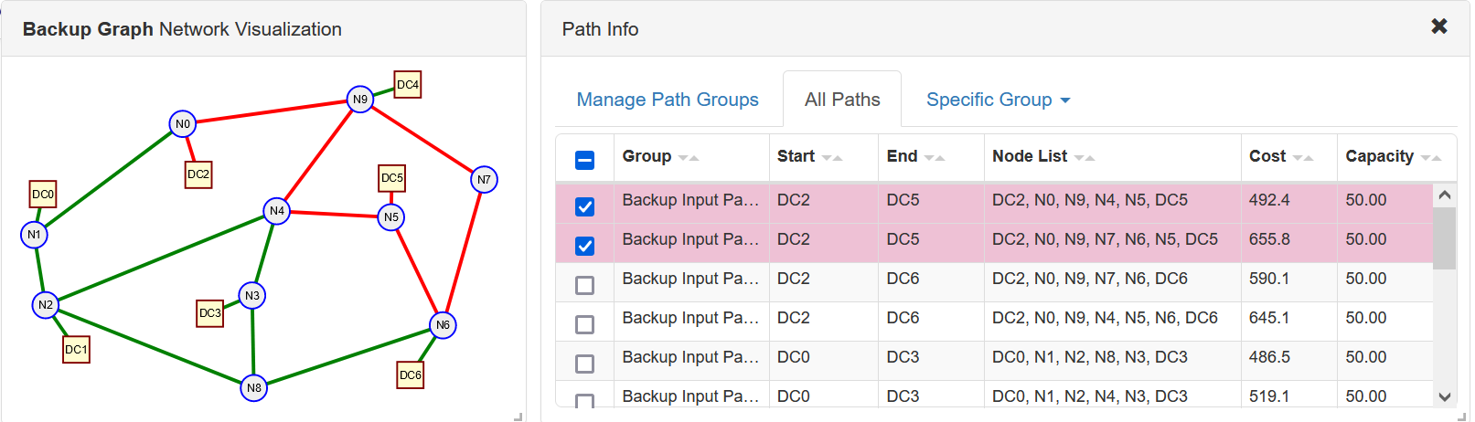
}The network model and the input paths can be visualized by copying and pasting the data above into our ComNetViz App. For example in Figure 3 we show the two paths between DC2 and DC5 highlighted.
The resulting problem formulation had 672 variables and 1251 constraints. Typical number crunching times with different $\alpha$ values and different link capacities were around 0.043 seconds with data loading times around 0.15 seconds.
In our first demonstration optimization we reduced the link capacities to 25 units and set $\alpha = 100$. With these parameters data center costs were emphasized over network costs though with the reduced capacities more "backup time periods" were required to meet the requirements.
{
  "id": "Backup Solution Paths A100_2",
  "desc": "Solution Paths for the Data Center backup example alpha = 100, link capacities 25",
  "pathList": [
    {
      "load": 13.0,
      "cost": 590.1,
      "nodeList": ["DC2", "N0", "N9", "N7", "N6", "DC6"],
      "time": 9
    },
    {
      "load": 7.0,
      "cost": 590.1,
      "nodeList": ["DC2", "N0", "N9", "N7", "N6", "DC6"],
      "time": 10
    },
    {
      "load": 25.0,
      "cost": 590.1,
      "nodeList": ["DC2", "N0", "N9", "N7", "N6", "DC6"],
      "time": 16
    },
    {
      "load": 25.0,
      "cost": 590.1,
      "nodeList": ["DC2", "N0", "N9", "N7", "N6", "DC6"],
      "time": 17
    },
    {
      "load": 25.0,
      "cost": 590.1,
      "nodeList": ["DC2", "N0", "N9", "N7", "N6", "DC6"],
      "time": 18
    },
    {
      "load": 25.0,
      "cost": 590.1,
      "nodeList": ["DC2", "N0", "N9", "N7", "N6", "DC6"],
      "time": 19
    },
    {
      "load": 25.0,
      "cost": 590.1,
      "nodeList": ["DC2", "N0", "N9", "N7", "N6", "DC6"],
      "time": 20
    },
    {
      "load": 25.0,
      "cost": 590.1,
      "nodeList": ["DC2", "N0", "N9", "N7", "N6", "DC6"],
      "time": 21
    },
    {
      "load": 25.0,
      "cost": 590.1,
      "nodeList": ["DC2", "N0", "N9", "N7", "N6", "DC6"],
      "time": 22
    },
    {
      "load": 25.0,
      "cost": 590.1,
      "nodeList": ["DC2", "N0", "N9", "N7", "N6", "DC6"],
      "time": 23
    },
    {
      "load": 25.0,
      "cost": 631.0,
      "nodeList": ["DC0", "N1", "N2", "N8", "N6", "DC6"],
      "time": 0
    },
    {
      "load": 25.0,
      "cost": 631.0,
      "nodeList": ["DC0", "N1", "N2", "N8", "N6", "DC6"],
      "time": 1
    },
    {
      "load": 25.0,
      "cost": 631.0,
      "nodeList": ["DC0", "N1", "N2", "N8", "N6", "DC6"],
      "time": 2
    },
    {
      "load": 25.0,
      "cost": 631.0,
      "nodeList": ["DC0", "N1", "N2", "N8", "N6", "DC6"],
      "time": 3
    },
    {
      "load": 25.0,
      "cost": 631.0,
      "nodeList": ["DC0", "N1", "N2", "N8", "N6", "DC6"],
      "time": 4
    },
    {
      "load": 25.0,
      "cost": 631.0,
      "nodeList": ["DC0", "N1", "N2", "N8", "N6", "DC6"],
      "time": 5
    },
    {
      "load": 25.0,
      "cost": 631.0,
      "nodeList": ["DC0", "N1", "N2", "N8", "N6", "DC6"],
      "time": 6
    },
    {
      "load": 25.0,
      "cost": 631.0,
      "nodeList": ["DC0", "N1", "N2", "N8", "N6", "DC6"],
      "time": 7
    },
    {
      "load": 25.0,
      "cost": 631.0,
      "nodeList": ["DC0", "N1", "N2", "N8", "N6", "DC6"],
      "time": 8
    },
    {
      "load": 12.0,
      "cost": 631.0,
      "nodeList": ["DC0", "N1", "N2", "N8", "N6", "DC6"],
      "time": 9
    },
    {
      "load": 25.0,
      "cost": 565.4,
      "nodeList": ["DC1", "N2", "N4", "N9", "DC4"],
      "time": 0
    },
    {
      "load": 25.0,
      "cost": 565.4,
      "nodeList": ["DC1", "N2", "N4", "N9", "DC4"],
      "time": 1
    },
    {
      "load": 25.0,
      "cost": 565.4,
      "nodeList": ["DC1", "N2", "N4", "N9", "DC4"],
      "time": 2
    },
    {
      "load": 25.0,
      "cost": 565.4,
      "nodeList": ["DC1", "N2", "N4", "N9", "DC4"],
      "time": 3
    },
    {
      "load": 25.0,
      "cost": 565.4,
      "nodeList": ["DC1", "N2", "N4", "N9", "DC4"],
      "time": 4
    },
    {
      "load": 25.0,
      "cost": 565.4,
      "nodeList": ["DC1", "N2", "N4", "N9", "DC4"],
      "time": 5
    },
    {
      "load": 25.0,
      "cost": 565.4,
      "nodeList": ["DC1", "N2", "N4", "N9", "DC4"],
      "time": 6
    },
    {
      "load": 25.0,
      "cost": 565.4,
      "nodeList": ["DC1", "N2", "N4", "N9", "DC4"],
      "time": 7
    },
    {
      "load": 25.0,
      "cost": 565.4,
      "nodeList": ["DC1", "N2", "N4", "N9", "DC4"],
      "time": 8
    },
    {
      "load": 12.0,
      "cost": 565.4,
      "nodeList": ["DC1", "N2", "N4", "N9", "DC4"],
      "time": 9
    },
    {
      "load": 18.0,
      "cost": 584.2,
      "nodeList": ["DC1", "N2", "N8", "N6", "DC6"],
      "time": 10
    },
    {
      "load": 25.0,
      "cost": 584.2,
      "nodeList": ["DC1", "N2", "N8", "N6", "DC6"],
      "time": 11
    },
    {
      "load": 25.0,
      "cost": 584.2,
      "nodeList": ["DC1", "N2", "N8", "N6", "DC6"],
      "time": 12
    },
    {
      "load": 25.0,
      "cost": 584.2,
      "nodeList": ["DC1", "N2", "N8", "N6", "DC6"],
      "time": 13
    },
    {
      "load": 25.0,
      "cost": 584.2,
      "nodeList": ["DC1", "N2", "N8", "N6", "DC6"],
      "time": 14
    },
    {
      "load": 25.0,
      "cost": 584.2,
      "nodeList": ["DC1", "N2", "N8", "N6", "DC6"],
      "time": 15
    }
  ]
}
In Figure 4 we show our visualization app with these solution paths loaded sorted by "time period" in which the paths are used.
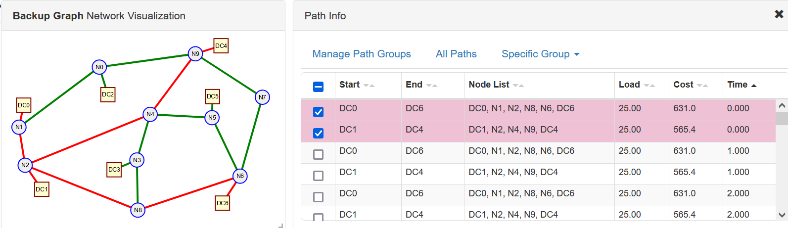
In our second demonstration optimization we reduced the link capacities to 15 units and set $\alpha = 1$ to emphasize network costs over data center costs.
{
  "id": "Backup Solution Paths A1_3",
  "desc": "Solution Paths for the Data Center backup example alpha = 1, link capacities 16",
  "pathList": [
    {
      "load": 15.999999999999998,
      "cost": 492.4,
      "nodeList": ["DC2", "N0", "N9", "N4", "N5", "DC5"],
      "time": 0
    },
    {
      "load": 16.000000000000004,
      "cost": 492.4,
      "nodeList": ["DC2", "N0", "N9", "N4", "N5", "DC5"],
      "time": 1
    },
    {
      "load": 16.000000000000007,
      "cost": 492.4,
      "nodeList": ["DC2", "N0", "N9", "N4", "N5", "DC5"],
      "time": 2
    },
    {
      "load": 16.000000000000004,
      "cost": 492.4,
      "nodeList": ["DC2", "N0", "N9", "N4", "N5", "DC5"],
      "time": 3
    },
    {
      "load": 4.999999999999696,
      "cost": 492.4,
      "nodeList": ["DC2", "N0", "N9", "N4", "N5", "DC5"],
      "time": 4
    },
    {
      "load": 4.000000000000205,
      "cost": 492.4,
      "nodeList": ["DC2", "N0", "N9", "N4", "N5", "DC5"],
      "time": 7
    },
    {
      "load": 16.0,
      "cost": 492.4,
      "nodeList": ["DC2", "N0", "N9", "N4", "N5", "DC5"],
      "time": 12
    },
    {
      "load": 3.0000000000001976,
      "cost": 492.4,
      "nodeList": ["DC2", "N0", "N9", "N4", "N5", "DC5"],
      "time": 13
    },
    {
      "load": 16.000000000000014,
      "cost": 492.4,
      "nodeList": ["DC2", "N0", "N9", "N4", "N5", "DC5"],
      "time": 14
    },
    {
      "load": 15.999999999999906,
      "cost": 492.4,
      "nodeList": ["DC2", "N0", "N9", "N4", "N5", "DC5"],
      "time": 15
    },
    {
      "load": 15.999999999999998,
      "cost": 492.4,
      "nodeList": ["DC2", "N0", "N9", "N4", "N5", "DC5"],
      "time": 16
    },
    {
      "load": 15.999999999999998,
      "cost": 492.4,
      "nodeList": ["DC2", "N0", "N9", "N4", "N5", "DC5"],
      "time": 17
    },
    {
      "load": 15.999999999999998,
      "cost": 492.4,
      "nodeList": ["DC2", "N0", "N9", "N4", "N5", "DC5"],
      "time": 18
    },
    {
      "load": 16.000000000000014,
      "cost": 492.4,
      "nodeList": ["DC2", "N0", "N9", "N4", "N5", "DC5"],
      "time": 19
    },
    {
      "load": 15.999999999999998,
      "cost": 492.4,
      "nodeList": ["DC2", "N0", "N9", "N4", "N5", "DC5"],
      "time": 20
    },
    {
      "load": 15.999999999999982,
      "cost": 492.4,
      "nodeList": ["DC2", "N0", "N9", "N4", "N5", "DC5"],
      "time": 21
    },
    {
      "load": 11.000000000000307,
      "cost": 486.5,
      "nodeList": ["DC0", "N1", "N2", "N8", "N3", "DC3"],
      "time": 4
    },
    {
      "load": 16.00000000000001,
      "cost": 486.5,
      "nodeList": ["DC0", "N1", "N2", "N8", "N3", "DC3"],
      "time": 5
    },
    {
      "load": 15.999999999999995,
      "cost": 486.5,
      "nodeList": ["DC0", "N1", "N2", "N8", "N3", "DC3"],
      "time": 6
    },
    {
      "load": 15.999999999999995,
      "cost": 486.5,
      "nodeList": ["DC0", "N1", "N2", "N8", "N3", "DC3"],
      "time": 7
    },
    {
      "load": 15.999999999999988,
      "cost": 486.5,
      "nodeList": ["DC0", "N1", "N2", "N8", "N3", "DC3"],
      "time": 8
    },
    {
      "load": 15.999999999999995,
      "cost": 486.5,
      "nodeList": ["DC0", "N1", "N2", "N8", "N3", "DC3"],
      "time": 9
    },
    {
      "load": 16.0,
      "cost": 486.5,
      "nodeList": ["DC0", "N1", "N2", "N8", "N3", "DC3"],
      "time": 10
    },
    {
      "load": 15.999999999999996,
      "cost": 486.5,
      "nodeList": ["DC0", "N1", "N2", "N8", "N3", "DC3"],
      "time": 11
    },
    {
      "load": 12.999999999999801,
      "cost": 486.5,
      "nodeList": ["DC0", "N1", "N2", "N8", "N3", "DC3"],
      "time": 13
    },
    {
      "load": 16.0,
      "cost": 486.5,
      "nodeList": ["DC0", "N1", "N2", "N8", "N3", "DC3"],
      "time": 22
    },
    {
      "load": 15.999999999999988,
      "cost": 486.5,
      "nodeList": ["DC0", "N1", "N2", "N8", "N3", "DC3"],
      "time": 23
    },
    {
      "load": 15.999999999999998,
      "cost": 519.1,
      "nodeList": ["DC0", "N1", "N2", "N4", "N3", "DC3"],
      "time": 0
    },
    {
      "load": 15.999999999999998,
      "cost": 519.1,
      "nodeList": ["DC0", "N1", "N2", "N4", "N3", "DC3"],
      "time": 1
    },
    {
      "load": 15.999999999999998,
      "cost": 519.1,
      "nodeList": ["DC0", "N1", "N2", "N4", "N3", "DC3"],
      "time": 2
    },
    {
      "load": 15.999999999999998,
      "cost": 519.1,
      "nodeList": ["DC0", "N1", "N2", "N4", "N3", "DC3"],
      "time": 3
    },
    {
      "load": 4.999999999999695,
      "cost": 519.1,
      "nodeList": ["DC0", "N1", "N2", "N4", "N3", "DC3"],
      "time": 4
    },
    {
      "load": 11.000000000000307,
      "cost": 565.4,
      "nodeList": ["DC1", "N2", "N4", "N9", "DC4"],
      "time": 4
    },
    {
      "load": 15.99999999999999,
      "cost": 565.4,
      "nodeList": ["DC1", "N2", "N4", "N9", "DC4"],
      "time": 5
    },
    {
      "load": 16.000000000000004,
      "cost": 565.4,
      "nodeList": ["DC1", "N2", "N4", "N9", "DC4"],
      "time": 6
    },
    {
      "load": 11.999999999999785,
      "cost": 565.4,
      "nodeList": ["DC1", "N2", "N4", "N9", "DC4"],
      "time": 7
    },
    {
      "load": 16.000000000000004,
      "cost": 565.4,
      "nodeList": ["DC1", "N2", "N4", "N9", "DC4"],
      "time": 8
    },
    {
      "load": 15.99999999999999,
      "cost": 565.4,
      "nodeList": ["DC1", "N2", "N4", "N9", "DC4"],
      "time": 9
    },
    {
      "load": 15.99999999999999,
      "cost": 565.4,
      "nodeList": ["DC1", "N2", "N4", "N9", "DC4"],
      "time": 10
    },
    {
      "load": 16.0,
      "cost": 565.4,
      "nodeList": ["DC1", "N2", "N4", "N9", "DC4"],
      "time": 11
    },
    {
      "load": 12.999999999999801,
      "cost": 565.4,
      "nodeList": ["DC1", "N2", "N4", "N9", "DC4"],
      "time": 13
    },
    {
      "load": 16.000000000000004,
      "cost": 565.4,
      "nodeList": ["DC1", "N2", "N4", "N9", "DC4"],
      "time": 22
    },
    {
      "load": 15.999999999999998,
      "cost": 565.4,
      "nodeList": ["DC1", "N2", "N4", "N9", "DC4"],
      "time": 23
    },
    {
      "load": 16.0,
      "cost": 584.2,
      "nodeList": ["DC1", "N2", "N8", "N6", "DC6"],
      "time": 0
    },
    {
      "load": 16.0,
      "cost": 584.2,
      "nodeList": ["DC1", "N2", "N8", "N6", "DC6"],
      "time": 1
    },
    {
      "load": 15.999999999999986,
      "cost": 584.2,
      "nodeList": ["DC1", "N2", "N8", "N6", "DC6"],
      "time": 2
    },
    {
      "load": 16.0,
      "cost": 584.2,
      "nodeList": ["DC1", "N2", "N8", "N6", "DC6"],
      "time": 3
    },
    {
      "load": 4.999999999999695,
      "cost": 584.2,
      "nodeList": ["DC1", "N2", "N8", "N6", "DC6"],
      "time": 4
    },
    {
      "load": 16.000000000000004,
      "cost": 584.2,
      "nodeList": ["DC1", "N2", "N8", "N6", "DC6"],
      "time": 12
    },
    {
      "load": 3.0000000000002025,
      "cost": 584.2,
      "nodeList": ["DC1", "N2", "N8", "N6", "DC6"],
      "time": 13
    },
    {
      "load": 16.000000000000004,
      "cost": 584.2,
      "nodeList": ["DC1", "N2", "N8", "N6", "DC6"],
      "time": 14
    },
    {
      "load": 16.0,
      "cost": 584.2,
      "nodeList": ["DC1", "N2", "N8", "N6", "DC6"],
      "time": 15
    },
    {
      "load": 16.000000000000004,
      "cost": 584.2,
      "nodeList": ["DC1", "N2", "N8", "N6", "DC6"],
      "time": 16
    },
    {
      "load": 16.0,
      "cost": 584.2,
      "nodeList": ["DC1", "N2", "N8", "N6", "DC6"],
      "time": 17
    },
    {
      "load": 16.0,
      "cost": 584.2,
      "nodeList": ["DC1", "N2", "N8", "N6", "DC6"],
      "time": 18
    },
    {
      "load": 16.0,
      "cost": 584.2,
      "nodeList": ["DC1", "N2", "N8", "N6", "DC6"],
      "time": 19
    },
    {
      "load": 16.000000000000014,
      "cost": 584.2,
      "nodeList": ["DC1", "N2", "N8", "N6", "DC6"],
      "time": 20
    },
    {
      "load": 16.0,
      "cost": 584.2,
      "nodeList": ["DC1", "N2", "N8", "N6", "DC6"],
      "time": 21
    }
  ]
}
In Figure 4 we show a screenshot of our visualization app with these paths.
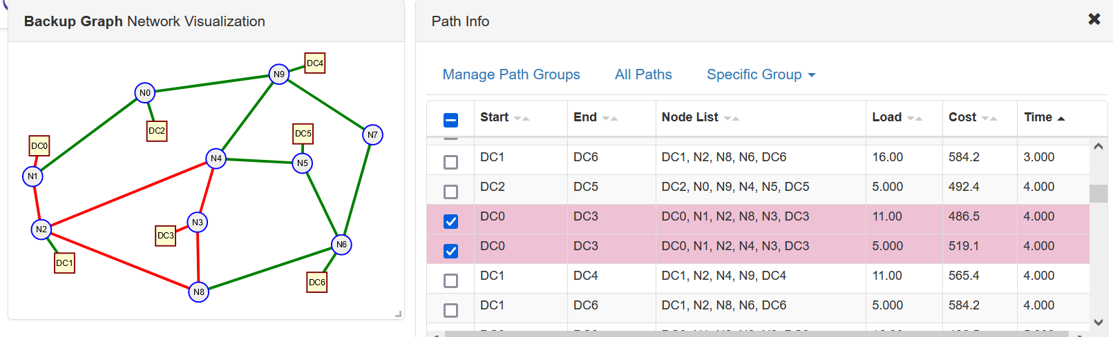
Further inspection of the paths with the app shows the lower cost (given) paths are used as much as possible. For example if you sort by "time" in the path table and look at time period 4 you will see DC0 communicating with DC3 over two different paths with the bulk of the traffic over the lower cost path. In addition during the same time period DC1 is talking to both DC4 and DC6 over the lower cost of the input paths.
References
[1] Dimitri P. Bertsekas, Network Optimization: Continuous and Discrete Models. Athena Scientific, 1998.
[2] D. Eppstein, "Finding the k Shortest Paths," SIAM J. Comput., vol. 28, no. 2, pp. 652-673, Jan. 1998.