Python/Pandas Fun with GPS Data, GPS Python GIS
Fun with GPS Data in Python
In this post we have some fun using a number of Python packages related to Geographic Information Systems (Wikipedia) (GIS). In it we will analyze GPS data from a nice hike. The same techniques can be applied to GPS track from any other fun activities such as walking, sailing, biking, etc… Or not to not so fun activities such as commuting, etc…
If you aren’t interested in programming in Python and just want a nice place to visulize GPS data for a hike visit Open Topo Map click on the gpx icon and load your GPX file.
We’ll be using a number of Python packages as detailed below. However, the point of this post is to show how to easily see some interesting results without reading through all the documentation! The GIS Python packages can rely on some native (C, C++) libraries and hence can be a bit tricky to install. A clear set of installation instructions from the GeoPandas project will get you everything you need.
- GeoPandas “GeoPandas is an open source project to make working with geospatial data in python easier. GeoPandas extends the datatypes used by pandas to allow spatial operations on geometric types. Geometric operations are performed by shapely. Geopandas further depends on fiona for file access and matplotlib for plotting.”
- Fiona “Fiona reads and writes geographic data files and thereby helps Python programmers integrate geographic information systems with other computer systems.”
- Pandas “pandas is a fast, powerful, flexible and easy to use open source data analysis and manipulation tool, built on top of the Python programming language.”
- Shapely “Manipulation and analysis of geometric objects in the Cartesian plane.”
Extra files: HikingAnalysis.ipynb and Hike-2022-06-30.gpx
import geopandas as gpd
import fiona
import shapely
import pandas as pd
import matplotlib.pyplot as plt
import numpy as np
Getting GPS Data
In this post we are going to work with GPS data in GPX (Wikipedia) format. GPX stands for “GPS Exchange Format” and is a widely used format to exchange GPS information. It can contain data as routes, tracks, and way points. From Wikipedia:
Conceptually, tracks are a record of where a person has been and routes are suggestions about where they might go in the future. For example, each point in a track may have a timestamp (because someone recorded where and when they were there), but the points in a route are unlikely to have timestamps (other than estimated trip duration) because route is a suggestion which might never have been traveled.
Get a GPX file or download mine to use. Set the file name below to point to your the file of your choice.
filename = r'C:\Greg_Home\GPS\Hikes\Hike-2022-06-30.gpx'Layers in GIS Files
The concept of map layers is ubiquitous in GIS systems and many file formats. Hence many libraries/packages utilize the concept in places where you might not expect it. Here we look at the layers of our GPX file with fiona:
fiona.listlayers(filename)['waypoints', 'routes', 'tracks', 'route_points', 'track_points']
Here we see that fiona understands that GPX files can contain routes, tracks and waypoints. We’ll see how the route_points and track_points are different from routes and tracks in a bit.
Track Layer
Let’s read in the track layer and take a look at where we have been in two lines of code!
gdf_tracks = gpd.read_file(filename, layer="tracks")
gdf_tracks.explore()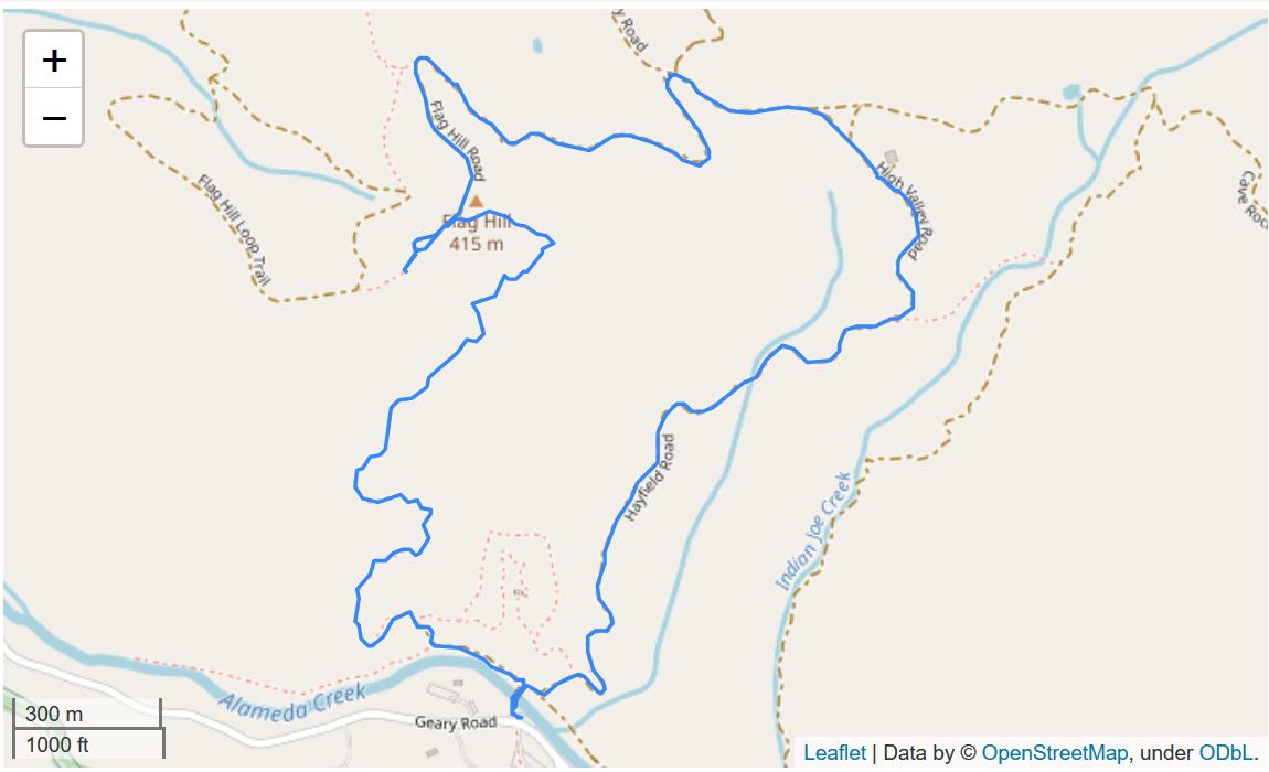
Let’s look at what the gdf_tracks object is and what it contains.
print(type(gdf_tracks))
print(f"length of gdf_tracks: {len(gdf_tracks)}")
print(type(gdf_tracks.iloc[0]))
print(gdf_tracks.iloc[0].keys())
print(type(gdf_tracks.iloc[0]["geometry"]))
<class 'geopandas.geodataframe.GeoDataFrame'>
length of gdf_tracks: 1
<class 'pandas.core.series.Series'>
Index(['name', 'cmt', 'desc', 'src', 'link1_href', 'link1_text', 'link1_type',
'link2_href', 'link2_text', 'link2_type', 'number', 'type', 'geometry'],
dtype='object')
<class 'shapely.geometry.multilinestring.MultiLineString'>
Getting the Shape
Hmm, that’s a lot of stuff. But the very last item is a
shapely.geometry. This has the actual coordinates of the track so lets
take a look.
Fiona/GeoPandas interprets tracks as a 2-dimensional multi-line string. No elevation information, time, or other information is kept.
mygeo_latlon = gdf_tracks.iloc[0]["geometry"]
mygeo_latlon
# Check the length of the multi-part geometry
print(f"Number of parts to the geometry: {len(mygeo_latlon.geoms)}")
print(type(mygeo_latlon.geoms[0]))
my_coords = mygeo_latlon.geoms[0].coords
print(f"length of coordinates: {len(my_coords)}")
print(my_coords[0:5])
Number of parts to the geometry: 1
<class 'shapely.geometry.linestring.LineString'>
length of coordinates: 6583
[(-121.830436667, 37.515446667), (-121.830446667, 37.515445), (-121.830446667, 37.515443333), (-121.830461667, 37.515443333), (-121.830473333, 37.515446667)]
So the “shape” is something called a “line string” and it contains an array of the coordinates. We see that the coordinates are in (longitude, latitude) format as record from the GPS device.
So for the tracks “layer” Fiona/GeoPandas gives us a 2-dimensional multi-line string. No elevation, time, or other information is kept.
# How long a hike, assume 1 coordinate a second
hike_hours = int(len(my_coords)/3600)
hike_minutes = int(len(my_coords)/60 % 60 + 0.5)
print(f"I was hiking for {hike_hours} hours and {hike_minutes} minutes")
I was hiking for 1 hours and 50 minutes
Simplifying Tracks Part 1
That’s a lot of track points. Can we reduce the number of points and have the shape look like the original? This turns out to be a common operatin and is supported by shapely:simplify. Here we are giving a tolerance value in decimal degrees.
simp_geo = mygeo_latlon.simplify(0.00001)
simp_geo
print(f"simplified number of coordinates: {len(simp_geo.coords)}")
print(simp_geo.coords[0:5])
simplified number of coordinates: 479
[(-121.830436667, 37.515446667), (-121.830461667, 37.515443333), (-121.830473333, 37.515446667), (-121.830485, 37.51545), (-121.830495, 37.51545)]
Distance Computations Raw
How far did I go? How do we compute distances from latitude and longitude based coordinates? From stack overflow I got this python implementation of the Wikipedia: Haversine formula. This results are in kilometers.
from math import cos, asin, sqrt, pi
# In kilometers
def distance(lat1, lon1, lat2, lon2):
    p = pi/180
    a = 0.5 - cos((lat2-lat1)*p)/2 + cos(lat1*p) * cos(lat2*p) * (1-cos((lon2-lon1)*p))/2
    return 12742 * asin(sqrt(a)) #2*R*asin...
meter2miles = 6.213712e-4
total = 0.0
coords = simp_geo.coords
for i in range(len(coords) - 1):
total += distance(coords[i][1], coords[i][0], coords[i+1][1], coords[i+1][0])
haver_total = total*1000*meter2miles
print(haver_total)3.7608495834710385
Distance from GeoPandas
Shouldn’t GeoPandas or Shapely be able to compute how far I hiked? Let try it.
gdf_tracks.lengthC:\Users\gregb\AppData\Local\Temp\ipykernel_24036\4027014172.py:1: UserWarning: Geometry is in a geographic CRS. Results from 'length' are likely incorrect. Use 'GeoSeries.to_crs()' to re-project geometries to a projected CRS before this operation.
gdf_tracks.length
0 0.063
dtype: float64
Hmm, that didn’t work. Let’s check the coordinate reference system CRS (Wikipedia).
gdf_tracks.crs<Geographic 2D CRS: EPSG:4326>
Name: WGS 84
Axis Info [ellipsoidal]:
- Lat[north]: Geodetic latitude (degree)
- Lon[east]: Geodetic longitude (degree)
Area of Use:
- name: World.
- bounds: (-180.0, -90.0, 180.0, 90.0)
Datum: World Geodetic System 1984 ensemble
- Ellipsoid: WGS 84
- Prime Meridian: Greenwich
Oh, we are using raw latitude and longitude. What we need is a map projection to take us from angle measurements in latitute and longitude to coordinates in something like miles or kilometers. For example the Web Mercator projection (EPSG:3857) is used for the maps of the OpenStreetMap-project and commercial products such as Bing Maps or Google Maps.
Let’s try setting the projection via GeoPandas:
gdf_tracks_3857 = gdf_tracks.to_crs(3857)meter2miles = 6.213712e-4
gdf_tracks_3857.length*meter2miles0 4.835374
dtype: float64
This is off by a mile from what we calculated from the Haversine formula. What happened?
Better Projection
We just hit upon one of the big issues that led to a proliferation of map projections over the last few centuries. No single map projection is good for all purposes. A general world wide projection like the Web Mercator that we used above will distort distances locally. See: Measuring Distances and Why Projections Matter.
For my hike it is better to use EPSG 32610.
Area of use: Between 126°W and 120°W, northern hemisphere between equator and 84°N, onshore and offshore. Canada - British Columbia (BC); Northwest Territories (NWT); Nunavut; Yukon. United States (USA) - Alaska (AK).
Coordinate system: Cartesian 2D CS. Axes: easting, northing (E,N). Orientations: east, north. UoM: meter
Let’s check that our lat and lon are within bounds then compute distances.
gdf_tracks.bounds| minx | miny | maxx | maxy | |
|---|---|---|---|---|
| 0 | -121.834233 | 37.515428 | -121.82141 | 37.52734 |
gdf_tracks_32610 = gdf_tracks.to_crs(32610)dist32610 = (gdf_tracks_32610.length*meter2miles)[0]
diff = haver_total - dist32610
print(f'Projection distance: {dist32610:.2f}, Haver distance: {haver_total:.2f}, diff: {diff:.2f}')Projection distance: 3.83, Haver distance: 3.76, diff: -0.07
This is much better and this is why a good local street map or topo map will use an appropriate projection, i.e., so you can get reasonably accurate distances by looking at the map.
Simplifying Tracks Part 2
Another advantage of using an appropriate projection is that we can now specify the tolerance use to simplify our tracks in a intuitive units, e.g., meters. Below we set the tolerance to simplify the hiking track to 3 meters. Note huge reduction in the number of points. This could be useful in producing routes to be followed from tracks.
# How many points when tolerance set to 3 meters?
len(gdf_tracks_32610.simplify(3.0).iloc[0].coords)
236
gdf_tracks_32610.simplify(3.0).explore()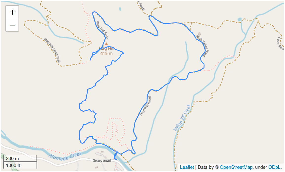
Note that it is good to use simplify when computing distances for slower moving activities since even if you are standing still GPS measurement noise will make it look as though you are moving.
# How many points do we get when tolerance set to 1 meter?
print(len(gdf_tracks_32610.simplify(1.0).iloc[0].coords))
print(gdf_tracks_32610.simplify(1.0).length*meter2miles)
480
0 3.760639
dtype: float64
Finally we take a peak at the coordinates in the ESPG 32610 projection. It turns out that these are in (x, y) meter pairs and hence distance calculations with them can just use Euclidean distance formulas.
coords32610 = gdf_tracks_32610.simplify(1.0).iloc[0].coords
print(coords32610[0:4])
[(603358.3633857827, 4152697.5049648797), (603356.1585678917, 4152697.1075925604), (603355.1229669412, 4152697.464678713), (603354.0872790867, 4152697.8216529465)]
Track Points Layer
In addition to latitude and longitude coordinates GPS track points can
contain other information such as elevation and time. For mountain hikes
I’m really interested in elevation information! This is where the
track_points layer comes in handy. It includes almost all the
information available in GPX format.
Let’s look at the column names (keys) that GeoPandas gives us and look at the first four rows of data.
gdf_points = gpd.read_file(filename, layer="track_points")print(gdf_points.keys())
gdf_points[0:4]Index(['track_fid', 'track_seg_id', 'track_seg_point_id', 'ele', 'time',
'course', 'speed', 'magvar', 'geoidheight', 'name', 'cmt', 'desc',
'src', 'url', 'urlname', 'sym', 'type', 'fix', 'sat', 'hdop', 'vdop',
'pdop', 'ageofdgpsdata', 'dgpsid', 'geometry'],
dtype='object')
| track_fid | track_seg_id | track_seg_point_id | ele | time | course | speed | magvar | geoidheight | name | ... | sym | type | fix | sat | hdop | vdop | pdop | ageofdgpsdata | dgpsid | geometry | |
|---|---|---|---|---|---|---|---|---|---|---|---|---|---|---|---|---|---|---|---|---|---|
| 0 | 0 | 0 | 0 | 99.0 | 2022-06-30 18:03:22+00:00 | 209.800003 | 0.252078 | None | None | None | ... | None | None | 3d | 5 | 1.6 | None | None | None | None | POINT (-121.83044 37.51545) |
| 1 | 0 | 0 | 1 | 100.0 | 2022-06-30 18:03:25+00:00 | 315.200012 | 0.262367 | None | None | None | ... | None | None | 3d | 5 | 1.6 | None | None | None | None | POINT (-121.83045 37.51544) |
| 2 | 0 | 0 | 2 | 103.0 | 2022-06-30 18:04:05+00:00 | 0.000000 | 0.000000 | None | None | None | ... | None | None | 3d | 6 | 1.4 | None | None | None | None | POINT (-121.83045 37.51544) |
| 3 | 0 | 0 | 3 | 103.0 | 2022-06-30 18:04:06+00:00 | 291.200012 | 1.111200 | None | None | None | ... | None | None | 3d | 6 | 1.4 | None | None | None | None | POINT (-121.83046 37.51544) |
4 rows × 25 columns
GPX Point Data
So what is all this extra information?
- tracks can contain multiple track segments e.g., when a GPS unit’s data collection is turned on and off. Hence the track segment related information.
- Per GPX standard ele is the elevation in meters.
- Per GPX standard time is the date/time referenced to UTC
- course and speed are extensions permitted by GPX and I only see these from my GPS watch that I use for windsurfing, kitesurfing, and sometime use hiking.
- sat is the number of GPS satelites in view
- hdop, vdop, and pdop are related to GPS accuracy
Interactive Tracks with Elevation and Time
Let’s use this data along with GeoPandas ploting capability to get an interactive map that can show the local time and elevation for each point along our hike. To do this we’ll create new “columns” in our GeoPandas data frame with a localized time string and the height converted to feet.
Note that the map is “interactive” in the Jupyter notebook not on the web page where we just show a static image.
# Function to take a Pandas timestamp and convert it to
# a local time string.
def ts_local_time(ts):
    return str(ts.tz_convert(tz='US/Pacific').time())
meters2feet = 3.28084gdf_points["ltime"] = gdf_points["time"].apply(ts_local_time)
gdf_points["efeet"] = meters2feet*gdf_points["ele"]gdf_points[["efeet", "ltime", "geometry"]].explore()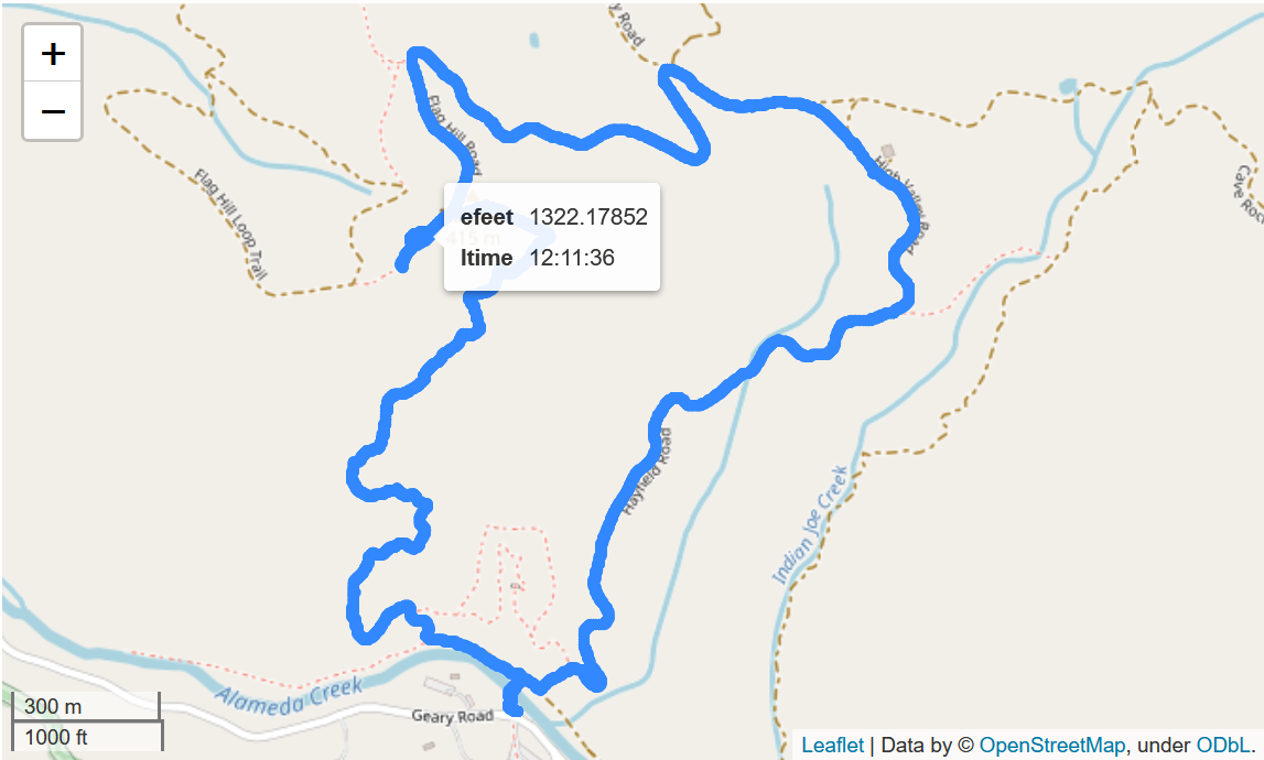
Check Vertical Progress
So how much vertical progress did our hike entail? By using the Pandas describe function show below we can see the minimum elevation was 275 feet and the maximum was 1325 feet.
gdf_points["efeet"].describe()count 6583.000000
mean 884.368538
std 315.168774
min 275.590560
25% 603.674560
50% 941.601080
75% 1141.732320
max 1325.459360
Name: efeet, dtype: float64
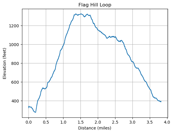
Elevation versus Distance
For hikes it is very nice to get a plot of elevation versus distance. Here we use GeoPandas and a the projection that gives us good distance measurements.
# Getting the bounds over all the points in the GeoPandas data frame.
gdf_points.total_bounds
array([-121.83423333, 37.51542833, -121.82141 , 37.52734 ])
# Set a good projection for distance computations
gdf_points32610 = gdf_points.to_crs(32610)
# Create a data frame from the differences between adjacent
# points and take a look at the first few entries.
diff_frame = pd.DataFrame({"xdiff": gdf_points32610.geometry.x.diff(),
"ydiff": gdf_points32610.geometry.y.diff()})
diff_frame[0:4]| xdiff | ydiff | |
|---|---|---|
| 0 | NaN | NaN |
| 1 | -0.881467 | -0.195939 |
| 2 | 0.002299 | -0.184952 |
| 3 | -1.325650 | -0.016481 |
# Compute the distance increment between adjacent points
dist_incrs = diff_frame.apply(lambda row: sqrt(row["xdiff"]**2 + row["ydiff"]**2), axis=1)
# Compute the accumulated distance up to each point
acc_dist = dist_incrs.cumsum()# Convert to miles and take a look
trk_miles = acc_dist*meter2miles
trk_miles0 NaN
1 0.000561
2 0.000676
3 0.001500
4 0.002180
...
6578 3.828678
6579 3.829488
6580 3.830083
6581 3.830595
6582 3.830778
Length: 6583, dtype: float64
# Replace the NaN with 0.0
trk_miles.iloc[0] = 0.0
# Get an array of heights in feet
trk_height = gdf_points32610.ele*meters2feet
# Plot it!
plt.plot(trk_miles, trk_height)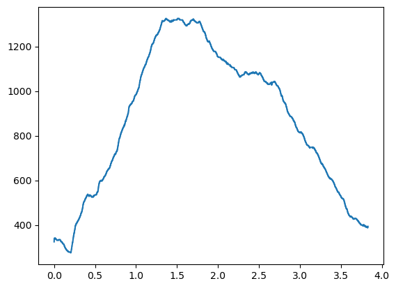
Projection Independent Elevation versus Distance
Alternatively we can do this in a way that is independent of the map projection via the Haversine formula that we used at the begining of this post. Here we will go to one of the underpinnings of Pandas which is the numpy package.
# Extract coordinates into a numpy array
coords = np.array([gdf_points.geometry.x.values,gdf_points.geometry.y.values])
# Take a look
print(coords[0][0], coords[1][0])
print(type(coords))-121.830436667 37.515446667
<class 'numpy.ndarray'>
# Get distance increments for an array of lat, lon values
# Uses def distance(lat1, lon1, lat2, lon2):
def dist_incrs(lon_lats):
    size = lon_lats.shape[1]
    incrs = np.zeros(size)
    for i in range(1, size):
        incrs[i] = 1000.0*distance(lon_lats[1][i-1], lon_lats[0][i-1],
                            lon_lats[1][i], lon_lats[0][i])
    return incrs
# compute distance increments
incrs2 = dist_incrs(coords)
# compute accumulated distance
cum_dist = incrs2.cumsum()*meter2miles
# get elevation in feet
elev = gdf_points.ele.values*meters2feet# Plot it nicely this time
fig, ax = plt.subplots()
ax.plot(cum_dist, elev)
ax.set(xlabel='Distance (miles)', ylabel='Elevation (feet)',
title='Flag Hill Loop')
plt.grid()
plt.show()